Topologies & Boundary Conditions
The grid topology fixes how neurons are arranged and, therefore, which neurons count
as neighbors during training. TorchSOM supports two topologies — "rectangular"
and "hexagonal" — and an optional periodic (toroidal) wrap for either. This guide
covers when to pick each and how to enable them. For the underlying geometry and the
grid-distance definitions, see 1. Grid Topology in
Basic Concepts.
Rectangular vs hexagonal
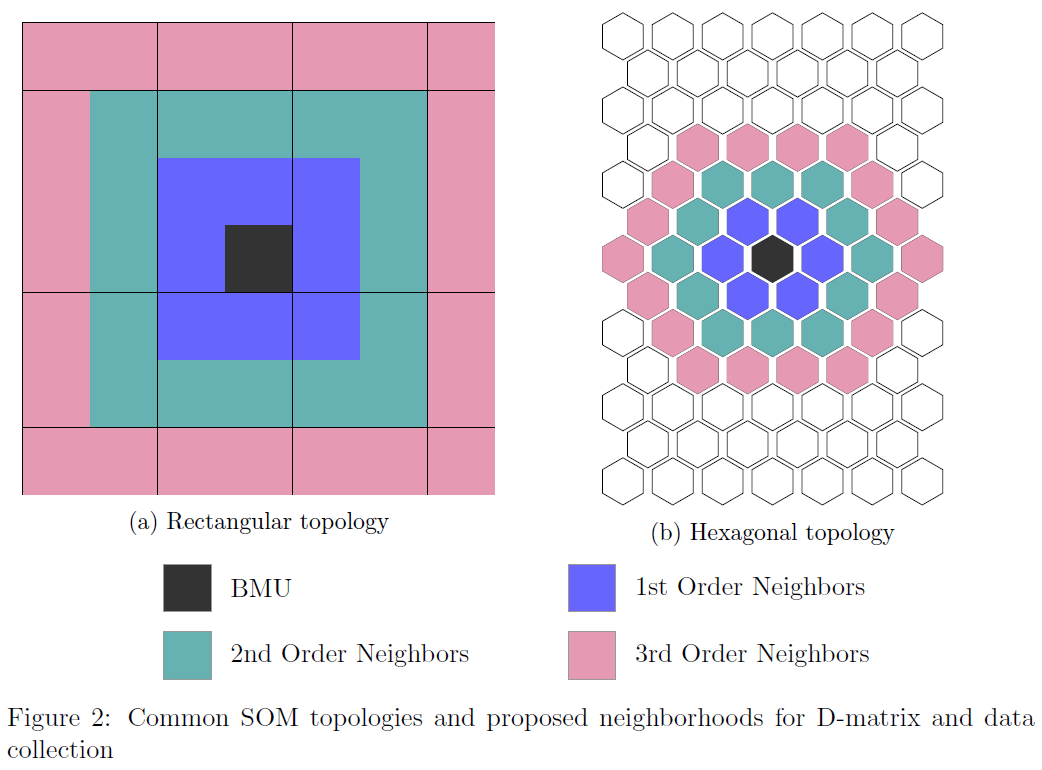
Rectangular |
Hexagonal |
|
|---|---|---|
Neighbors |
8 (Chebyshev block) |
6 (hop-distance rings) |
Order-\(o\) cell count |
\((2o+1)^2\) |
Hexagonal ring of radius \(o\) |
Reading the map |
Most intuitive; axis-aligned |
Uniform neighbor distances |
Typical use |
General-purpose default |
Lower topographic error; preferred for finer analysis |
Both topologies expose the same API; only the topology argument changes:
from torchsom import SOM

rect = SOM(x=25, y=15, num_features=4, topology="rectangular")
hexg = SOM(x=25, y=15, num_features=4, topology="hexagonal")
The Visualization Gallery gallery renders square cells for rectangular maps and hexagon cells for hexagonal maps automatically — your plotting code does not change.
Tip
If you are unsure, start rectangular for a quick, readable first pass, then switch to hexagonal when you want the lowest topographic error for a final map.
Periodic boundary conditions (toroidal maps)
By default the grid has edges, so corner and border neurons have fewer neighbors and
tend to be under-used. Setting pbc=True wraps opposite edges together, turning the
grid into a torus. Grid distances then use the minimum-image convention, so
neighborhoods wrap across boundaries and no neuron is disadvantaged by its position.
from torchsom import SOM

som = SOM(
    x=25,
    y=15,
    num_features=4,
    topology="hexagonal",
    pbc=True,               # wrap the lattice into a torus
)
When to enable PBC:
The input space has no natural boundary — cyclic or angular features (hour-of-day, wind direction, phase).
You want uniform neuron utilization and no edge artifacts on the U-matrix.
When to leave it off (the default):
The data has genuine extremes you want pushed to the map borders.
You need the most directly interpretable 2-D layout.
PBC works with both topologies and changes only the grid-distance computation; every other part of the API (training, visualization, clustering, JITL) is unaffected.
Effect on neighborhoods and JITL
The neighborhood order \(o\) (the neighborhood_order argument) sets how far the
discrete neighborhood extends — a \((2o+1)\times(2o+1)\) block on a rectangular
grid, or hop-distance rings on a hexagonal grid. The same order governs the
neighborhood used by Just-in-Time Learning sample retrieval. Under PBC these neighborhoods wrap
across edges, which matters when you rely on collect_samples near a boundary.
Next steps
Training — Decay schedules, initialization, and BMU search backends
Visualization Gallery — See both topologies rendered
1. Grid Topology — The grid-distance math behind PBC
Core API —
SOMconstructor reference