Iris — Classification¶

The Iris dataset (150 samples, 4 features, 3 species) is the classic first SOM. This tutorial trains a map, checks convergence, and reads the structure through the U-matrix, hit map, classification map, and component planes.

Note

Full runnable notebook: notebooks/iris.ipynb. The figures below are its outputs.

1. Load and standardize the data¶

The BMU search compares raw feature distances, so standardizing is essential.

import torch
from sklearn.datasets import load_iris
from sklearn.preprocessing import StandardScaler

bunch = load_iris()
features = torch.tensor(
    StandardScaler().fit_transform(bunch.data), dtype=torch.float32
)
targets = torch.tensor(bunch.target, dtype=torch.long)   # 0, 1, 2
feature_names = list(bunch.feature_names)

2. Train the SOM¶

from torchsom import SOM

som = SOM(
    x=25,
    y=15,
    num_features=features.shape[1],
    epochs=100,
    batch_size=16,
    sigma=1.45,
    learning_rate=0.95,
    neighborhood_order=3,
    topology="rectangular",
    initialization_mode="pca",
    random_seed=42,
)
som.initialize_weights(data=features, mode=som.initialization_mode)
q_errors, t_errors = som.fit(data=features)

3. Check convergence¶

from torchsom import SOMVisualizer

viz = SOMVisualizer(som=som)
viz.plot_training_errors(
    quantization_errors=q_errors, topographic_errors=t_errors
)

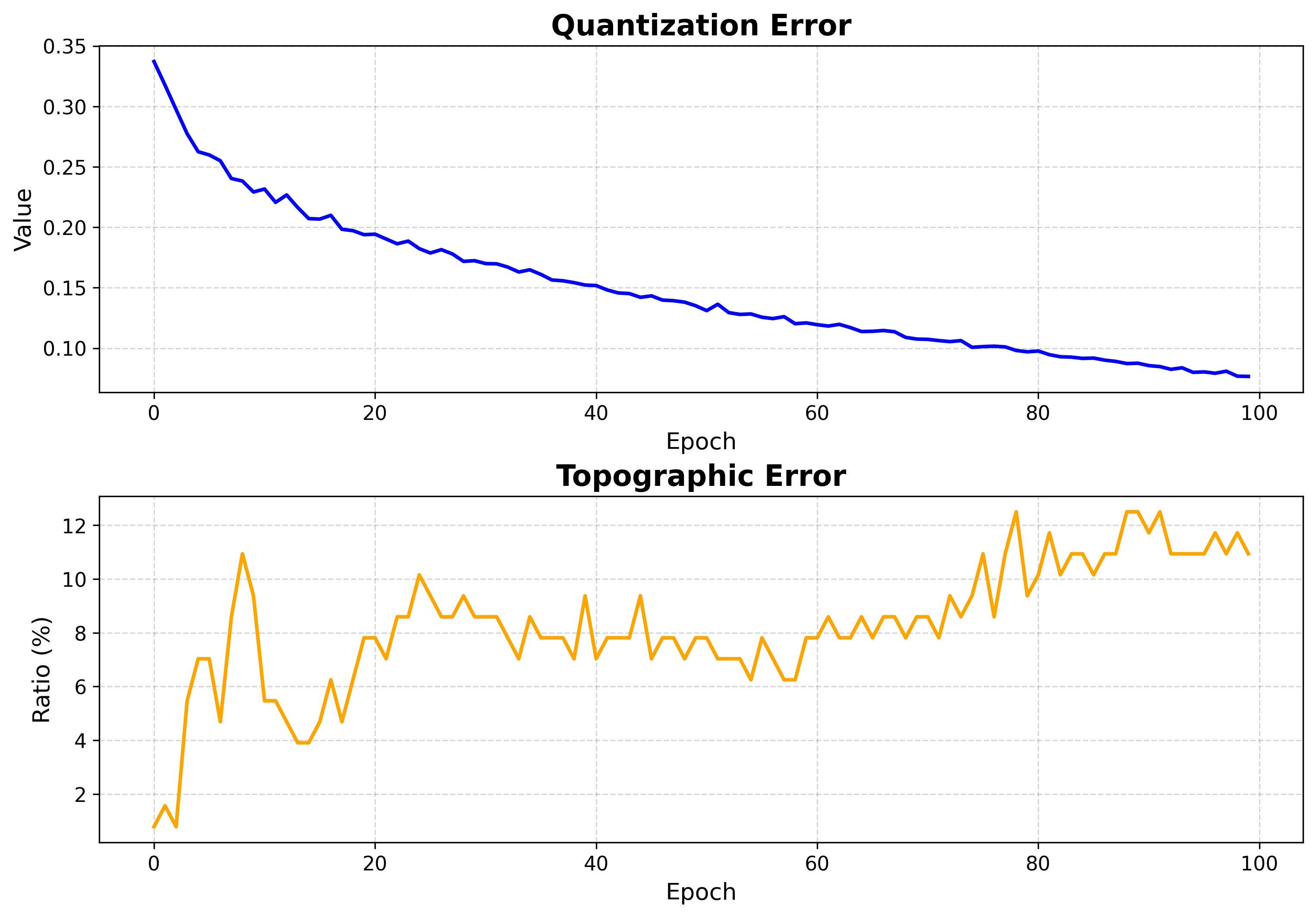
Both errors fall and flatten — training is long enough.

4. Inspect the map structure¶

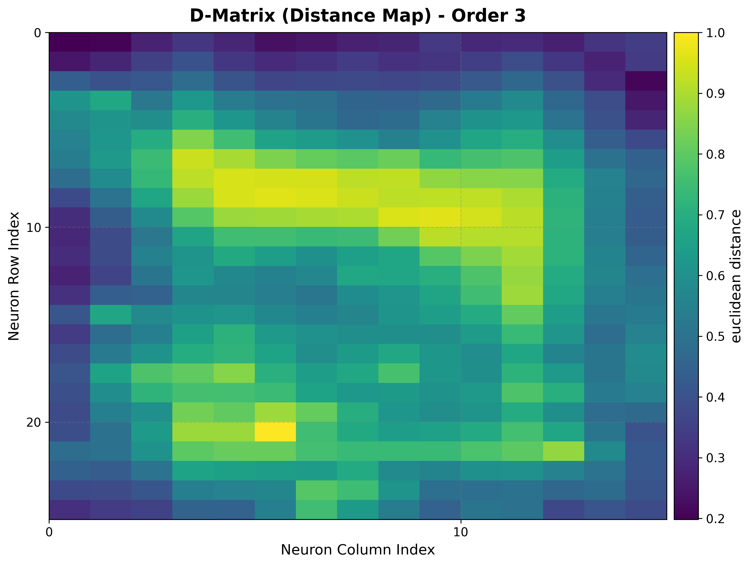
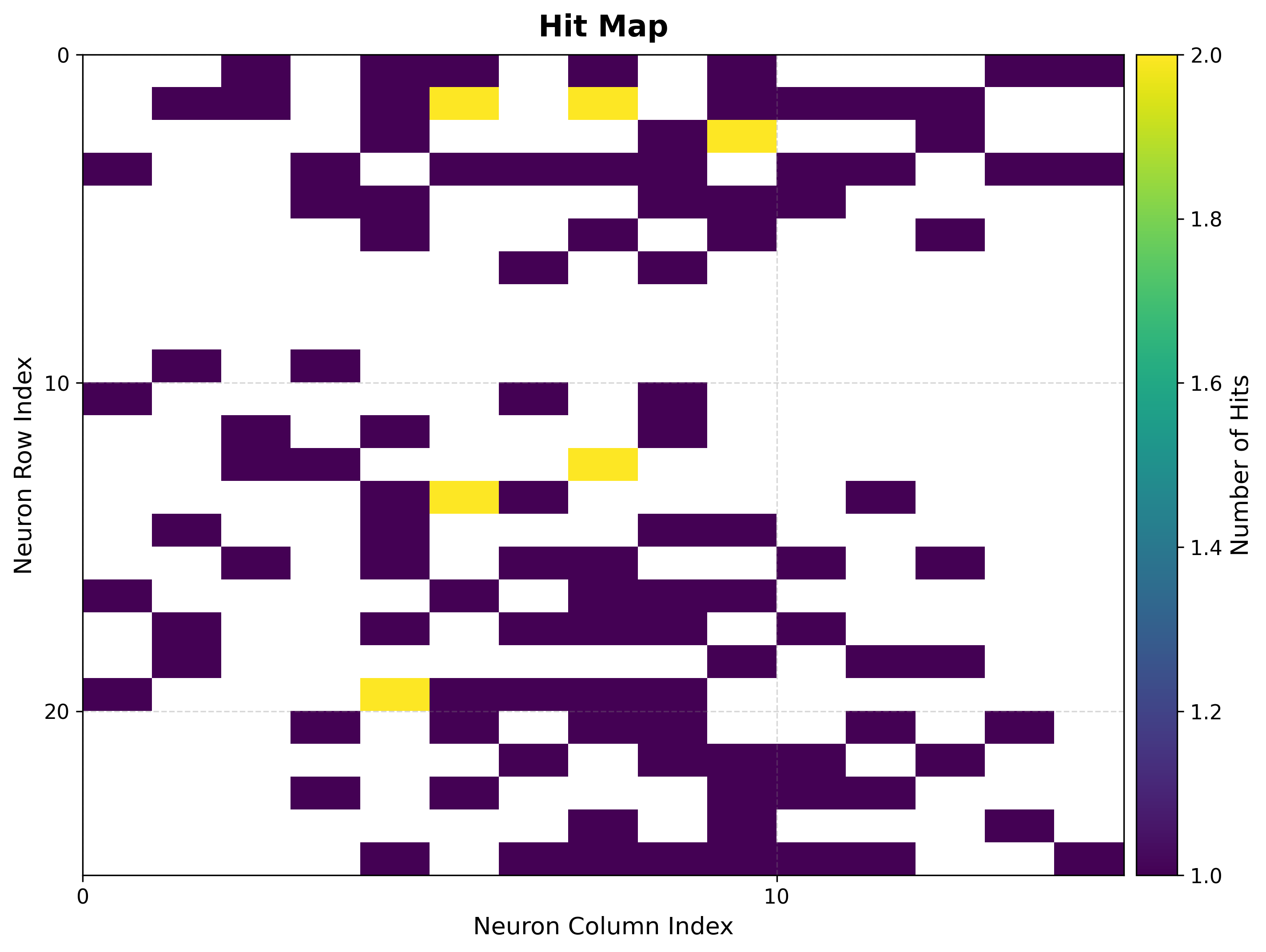
The U-matrix exposes cluster boundaries; the hit map shows where the data lands.

viz.plot_distance_map(
    distance_metric=som.distance_fn_name,
    neighborhood_order=som.neighborhood_order,
)
viz.plot_hit_map(data=features)

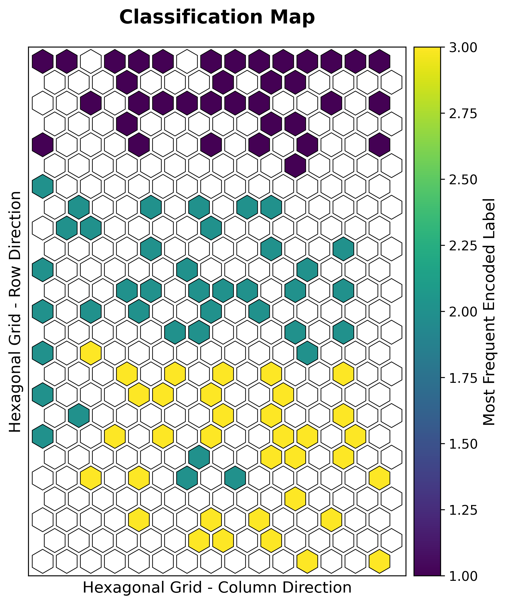
5. Classification map¶

Build the BMU→sample map once, then color each neuron by its dominant class.

bmus_map = som.build_map("bmus_data", data=features)
viz.plot_classification_map(
    bmus_data_map=bmus_map,
    data=features,
    target=targets,
    neighborhood_order=som.neighborhood_order,
)

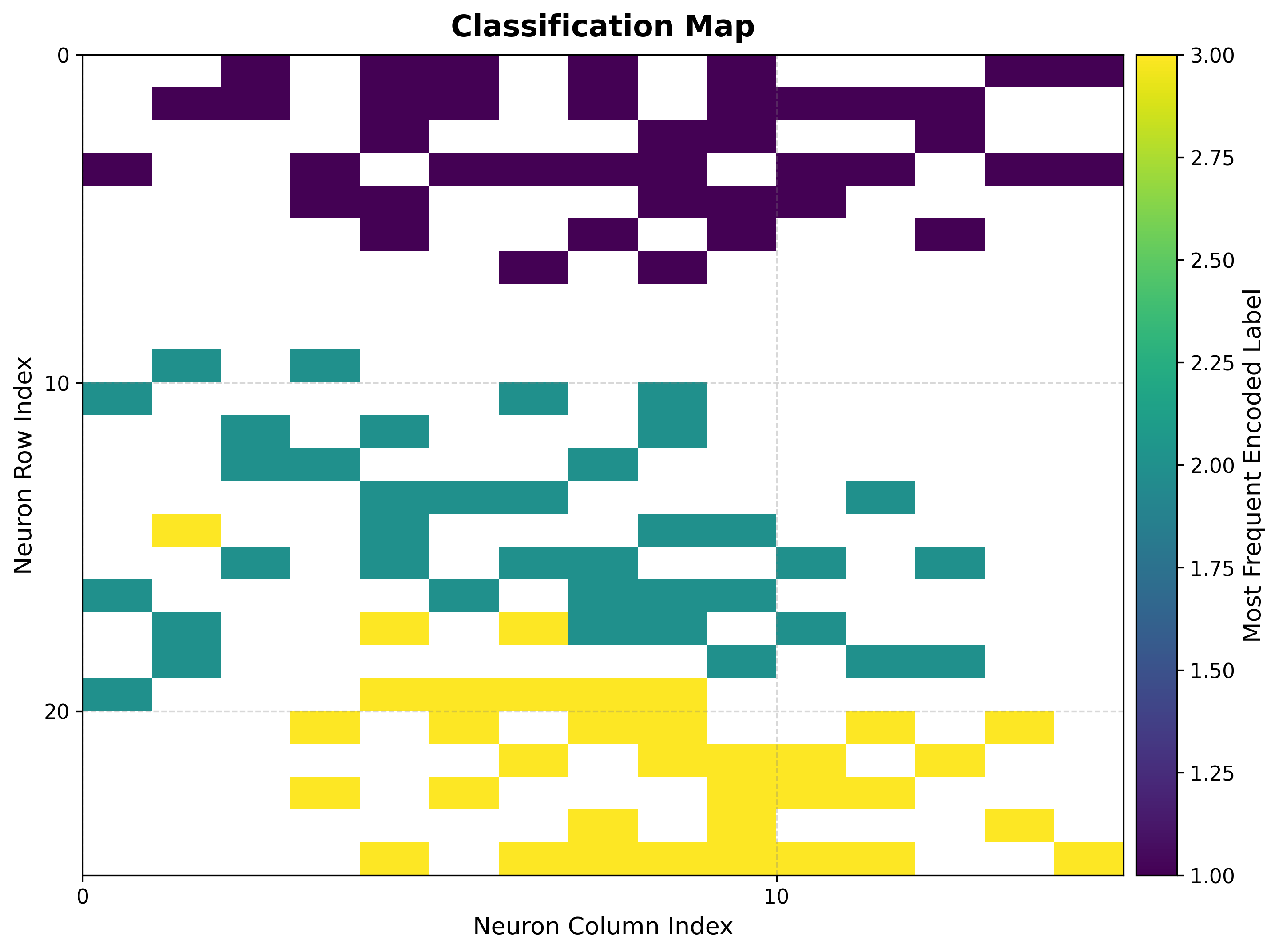
Iris setosa separates cleanly, while versicolor and virginica share a boundary — exactly the overlap known in this dataset, recovered here without supervision.

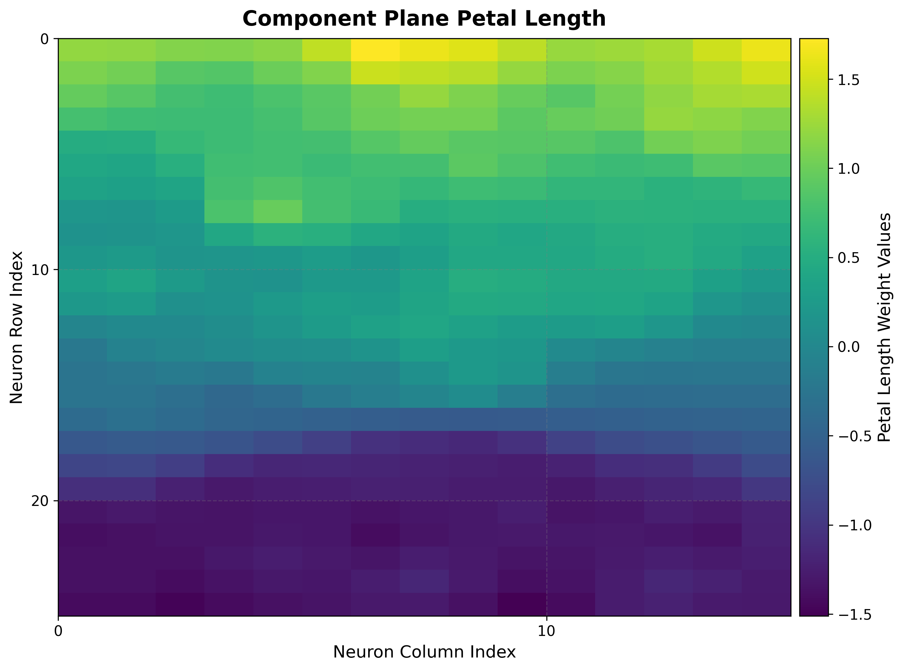
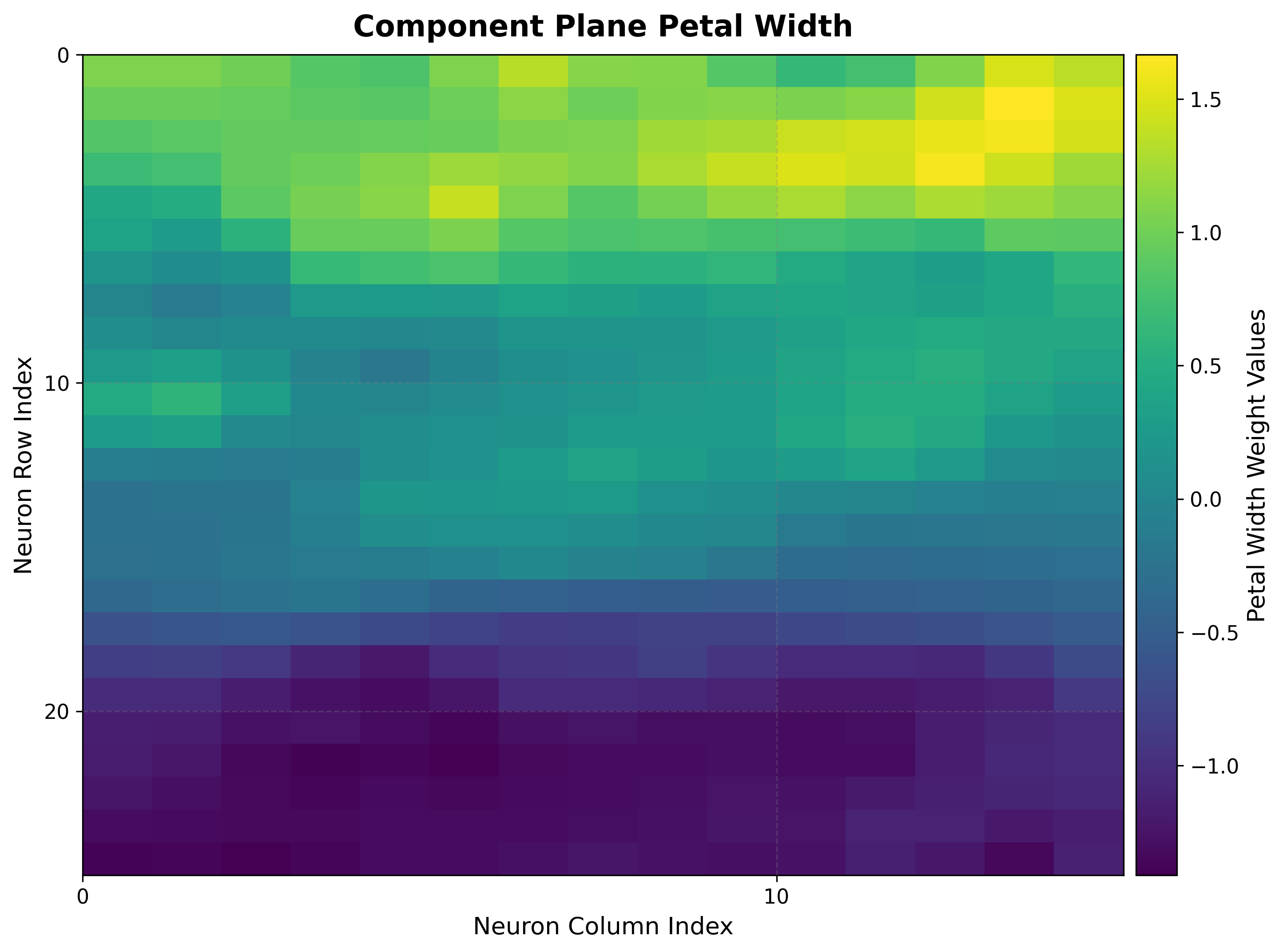
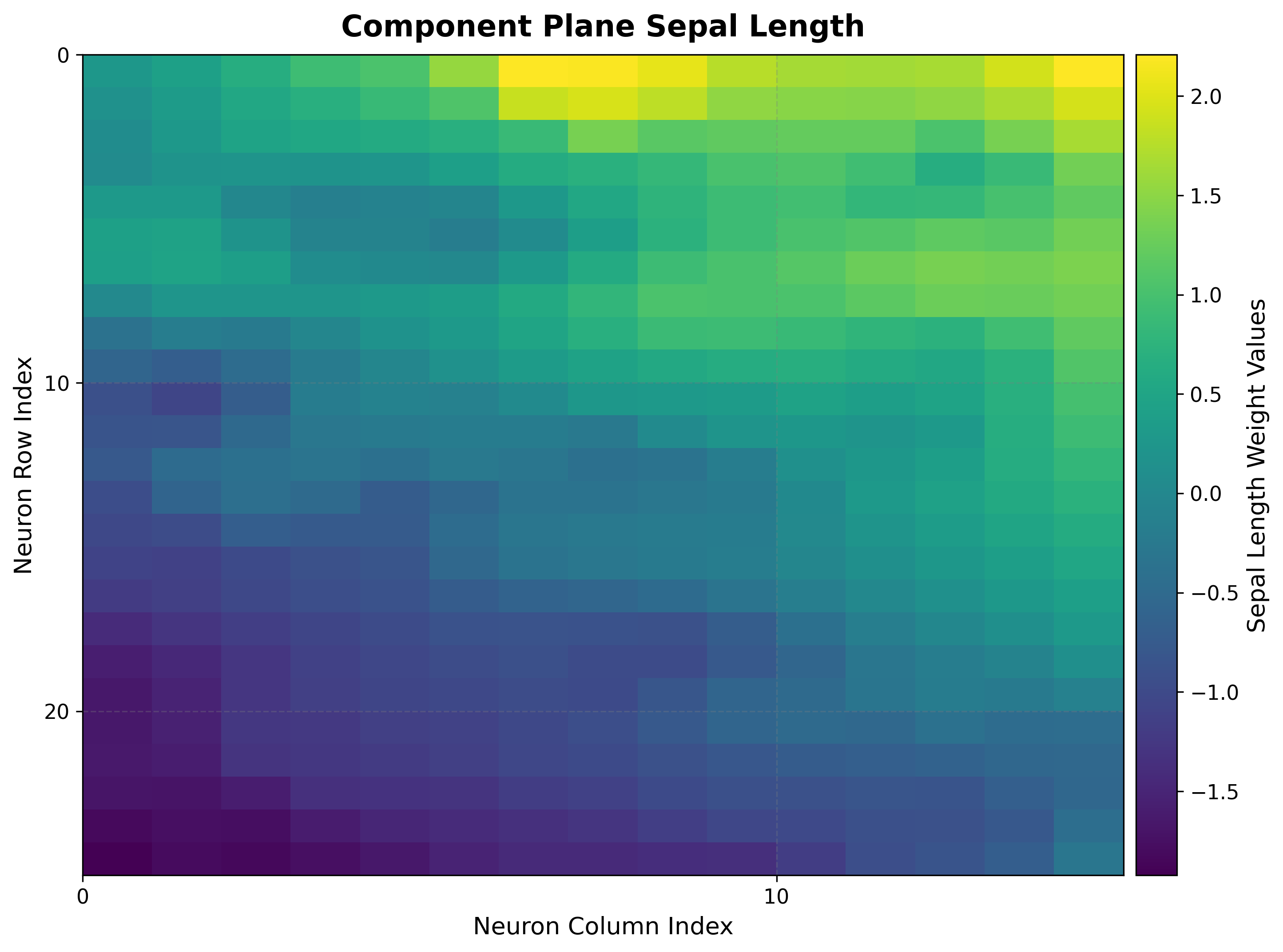
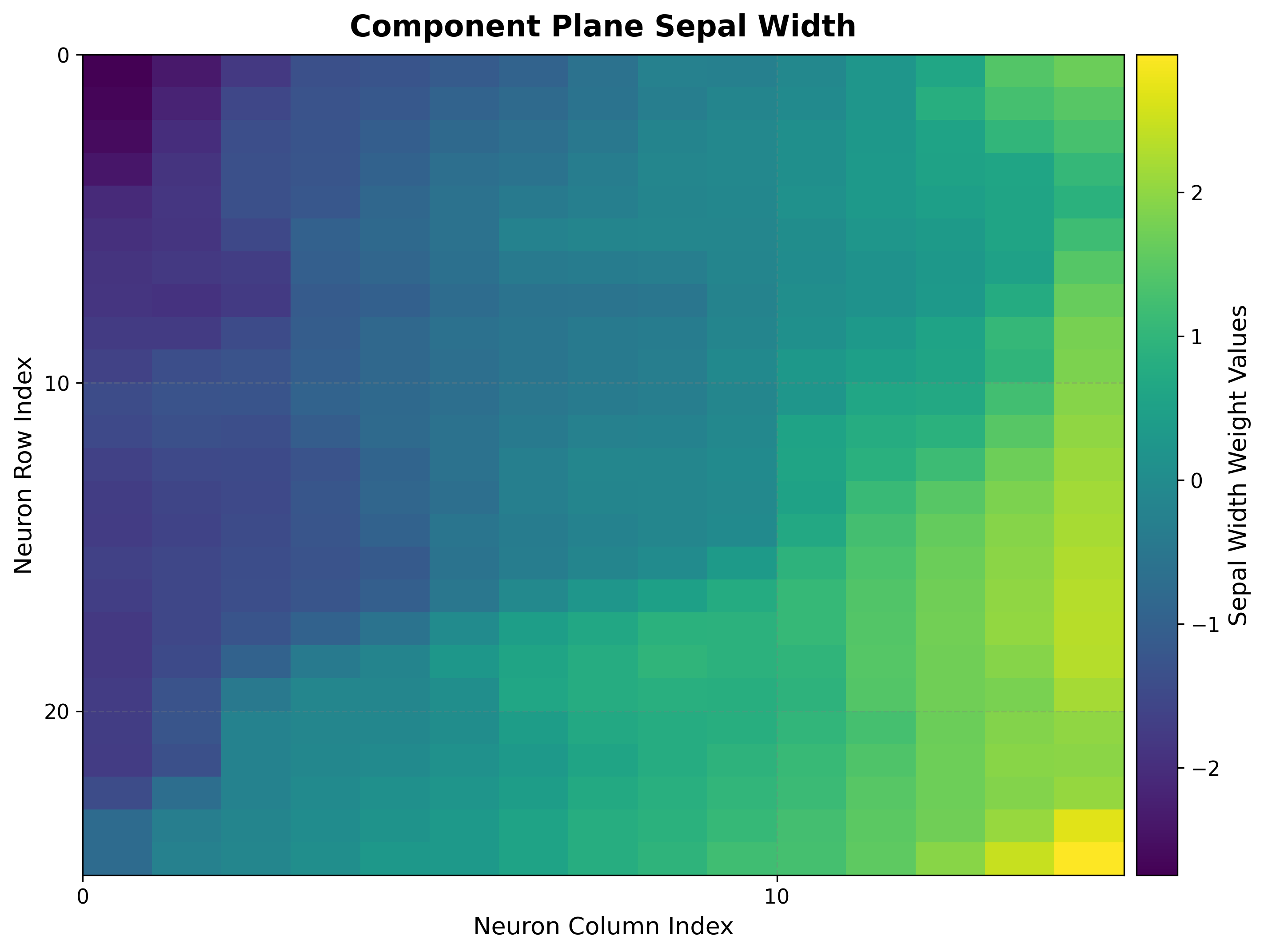
6. Component planes¶

One heat map per feature reveals which features drive the separation.

viz.plot_component_planes(component_names=feature_names)

Petal length and width vary together across the grid and align with the class regions, confirming they are the most discriminative features.

Hexagonal variant¶

Set topology="hexagonal" for the same analysis on a hexagonal grid; the visualizer renders hexagon cells automatically:

Iris classification map on a hexagonal grid

Next steps¶

Wine — Classification — A higher-dimensional classification example
Boston Housing — Regression — From classification to regression
Visualization Gallery — Every plot explained