Energy Efficiency — Multi-target Regression
The Energy Efficiency dataset (768 samples, 8 building-design features, 2 continuous targets) is a multi-target regression problem: each building has a Heating Load and a Cooling Load. This tutorial trains one SOM on the 8 features, then projects each target separately onto that same map to show how a single SOM supports multi-target analysis.
Note
Full runnable notebook: notebooks/energy_efficiency.ipynb. The figures below are its outputs.
1. Load and standardize the data
The first 8 columns are building-design features; the last two columns are the targets
(Heating Load, then Cooling Load). The BMU search compares raw feature
distances, so standardizing the features is essential.
import torch
import pandas as pd
from sklearn.preprocessing import StandardScaler

# energy_efficiency.csv ships in the repo
df = pd.read_csv("data/notebooks/energy_efficiency.csv")

feature_cols = df.columns[:8]
features = torch.tensor(
    StandardScaler().fit_transform(df[feature_cols].values), dtype=torch.float32
)
heating = torch.tensor(df["Heating Load"].values, dtype=torch.float32)
cooling = torch.tensor(df["Cooling Load"].values, dtype=torch.float32)
2. Train the SOM
from torchsom import SOM

som = SOM(
    x=25,
    y=15,
    num_features=features.shape[1],
    epochs=100,
    batch_size=16,
    sigma=1.45,
    learning_rate=0.95,
    neighborhood_order=3,
    topology="rectangular",
    initialization_mode="pca",
    random_seed=42,
)
som.initialize_weights(data=features, mode=som.initialization_mode)
q_errors, t_errors = som.fit(data=features)
3. Check convergence
from torchsom import SOMVisualizer

viz = SOMVisualizer(som=som)
viz.plot_training_errors(
    quantization_errors=q_errors, topographic_errors=t_errors
)
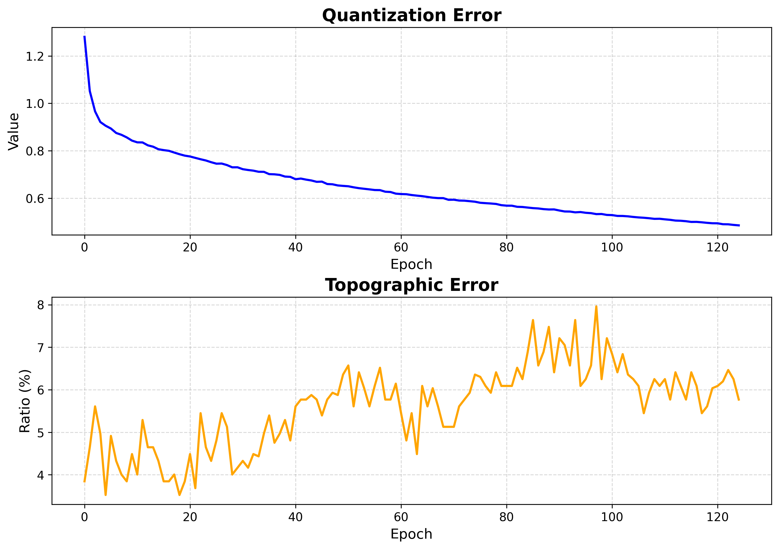
Both errors fall and flatten — training is long enough.
4. Inspect the map structure
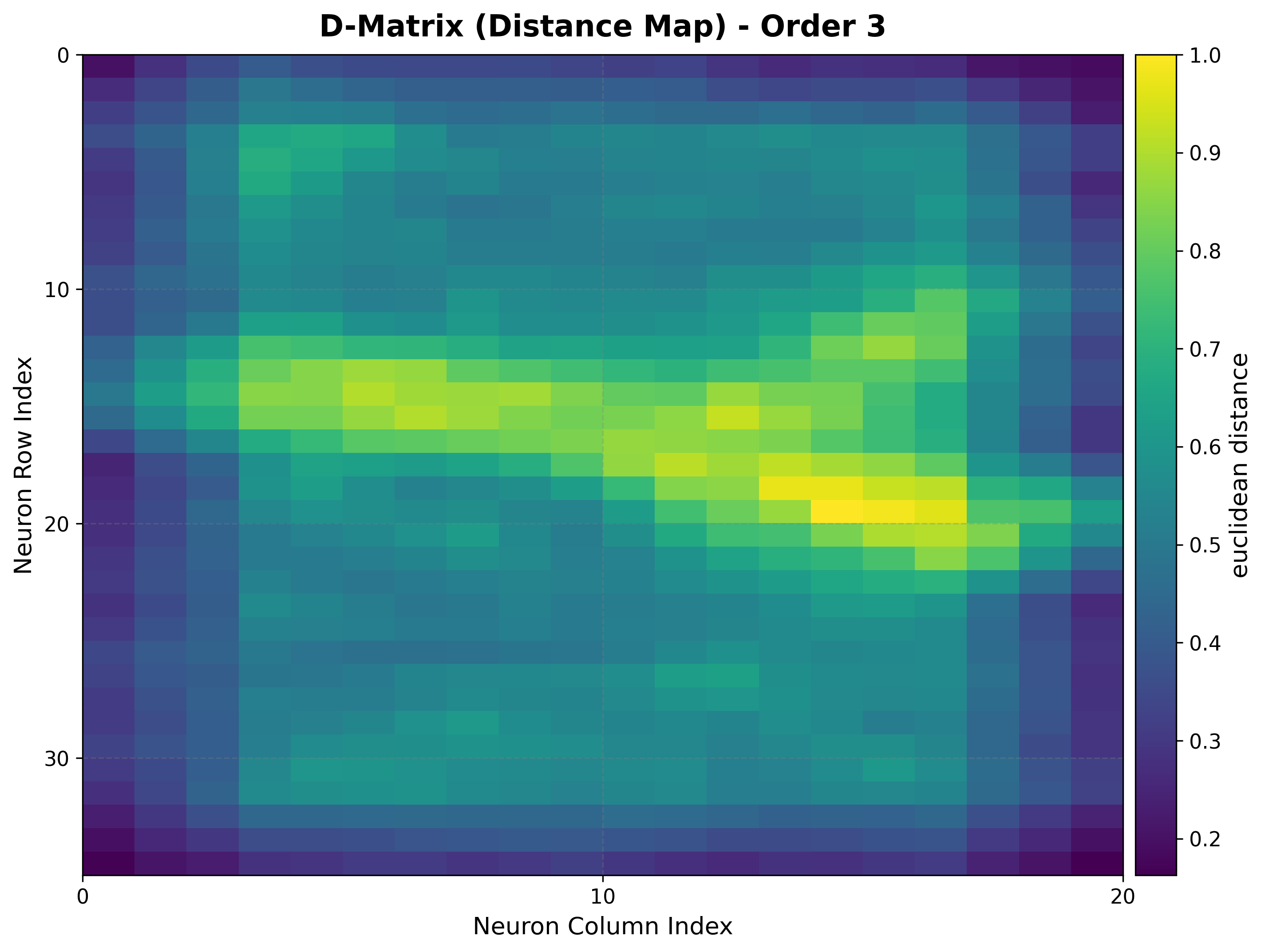
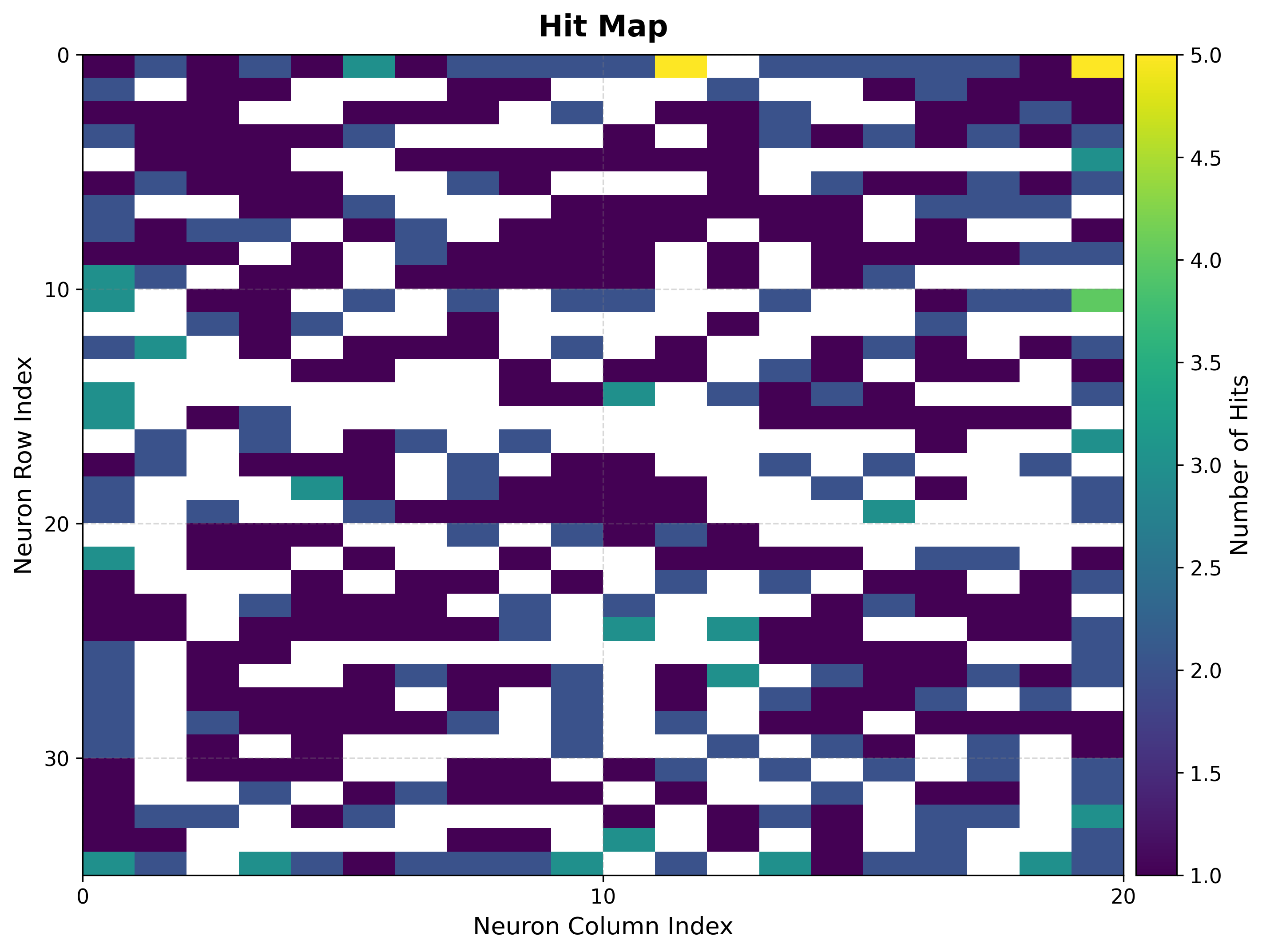
The U-matrix exposes cluster boundaries; the hit map shows where the data lands.
viz.plot_distance_map(
    distance_metric=som.distance_fn_name,
    neighborhood_order=som.neighborhood_order,
)
viz.plot_hit_map(data=features)
|
|
5. Heating load landscape
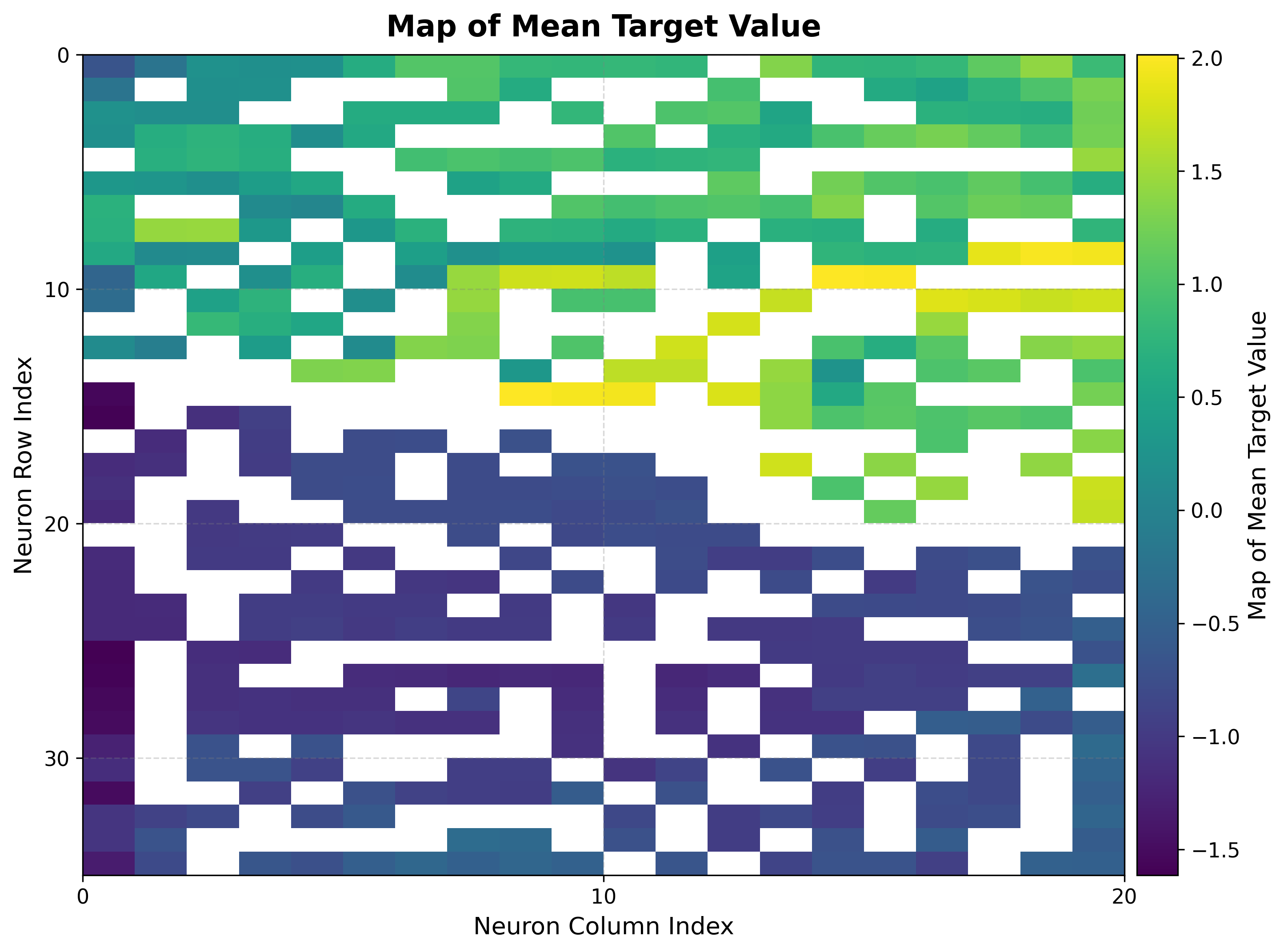
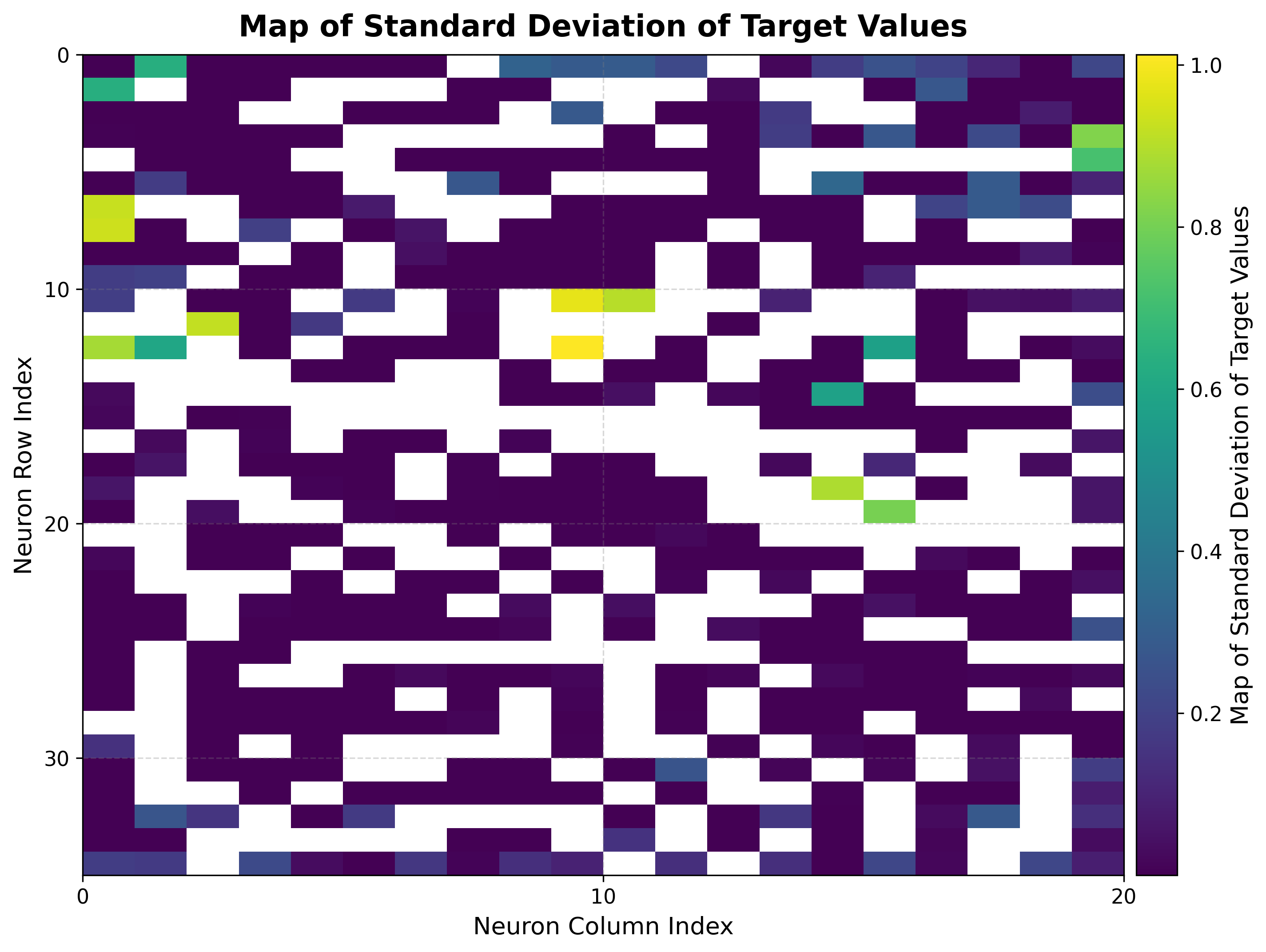
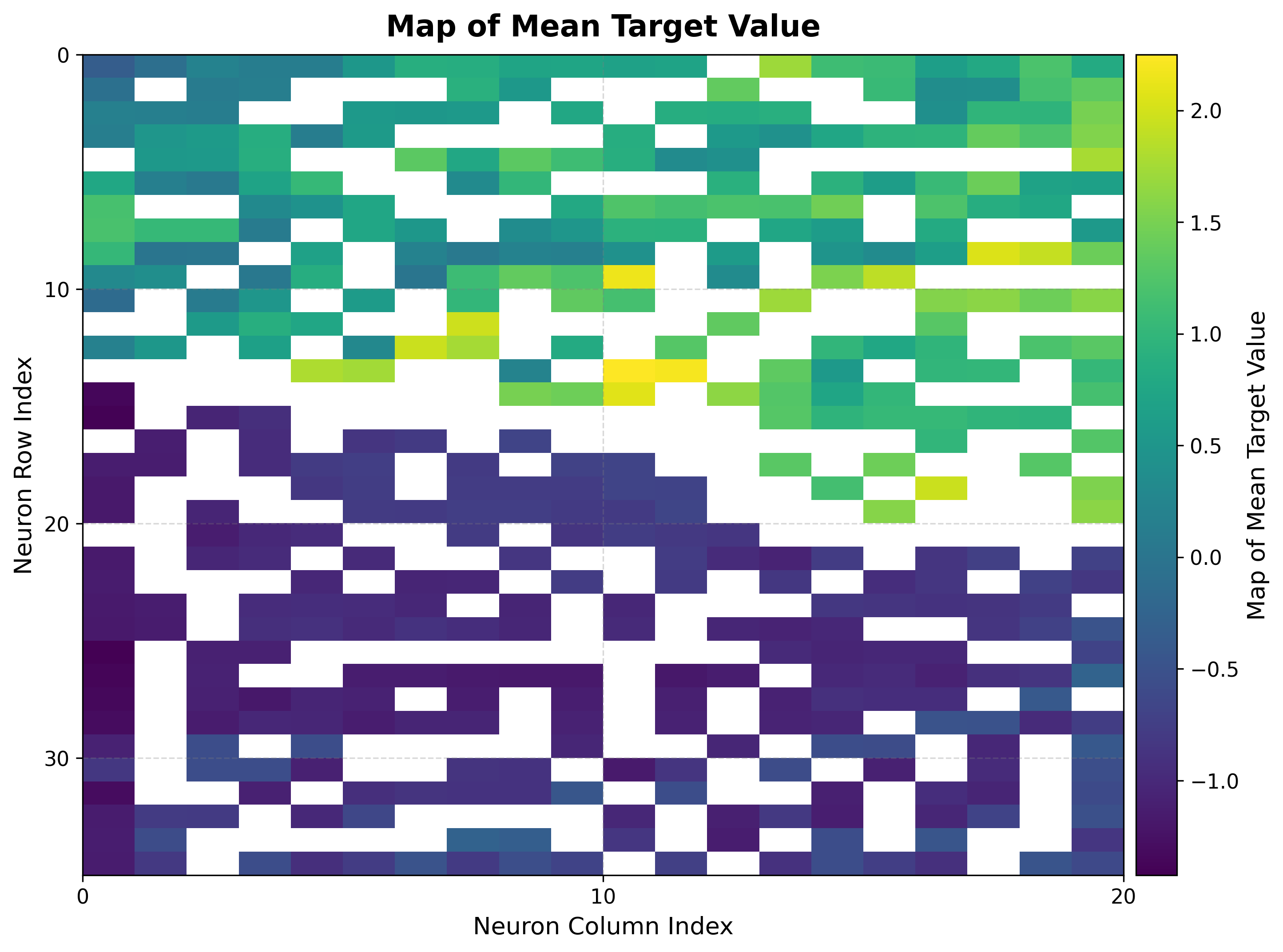
Build the BMU→sample map once, then reuse it for every target. Here it colors each neuron by the mean heating load of its samples, and by the standard deviation.
bmus_map = som.build_map("bmus_data", data=features)
viz.plot_metric_map(
    bmus_data_map=bmus_map,
    data=features,
    target=heating,
    reduction_parameter="mean",
)
viz.plot_metric_map(
    bmus_data_map=bmus_map,
    data=features,
    target=heating,
    reduction_parameter="std",
)
|
|
The mean map shows heating load varying smoothly across the grid, so nearby neurons hold buildings with similar loads. The std map reveals where the target is consistent: low values mark neurons whose samples share nearly the same heating load.
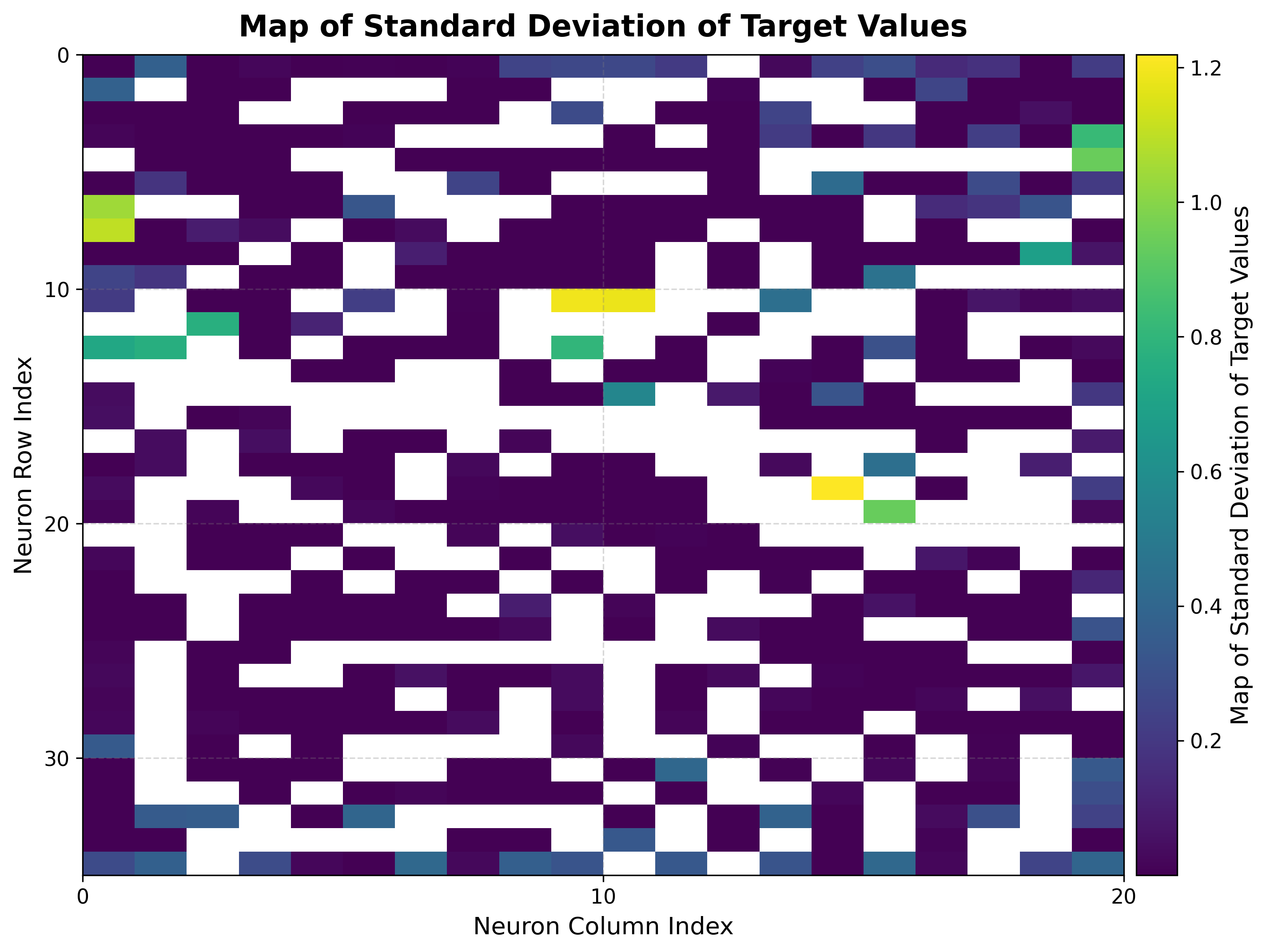
6. Cooling load landscape
The same bmus_map is reused — no retraining and no rebuild — now projecting the
cooling load onto the identical map.
viz.plot_metric_map(
    bmus_data_map=bmus_map,
    data=features,
    target=cooling,
    reduction_parameter="mean",
)
viz.plot_metric_map(
    bmus_data_map=bmus_map,
    data=features,
    target=cooling,
    reduction_parameter="std",
)
|
|
Heating and cooling loads produce similar but not identical landscapes on the same map: the two targets are correlated yet diverge in regions where building geometry affects them differently. The std map again marks where the cooling load is consistent within each neuron.
Next steps
Clustering — Synthetic Blobs — Group neurons into clusters
Boston Housing — Regression — Single-target regression on a SOM
Visualization Gallery — Every plot explained