Clustering
A trained SOM already organizes data into a topology-preserving grid. Clustering goes
one step further and groups the neurons themselves into a small number of regions,
turning the map into an explicit segmentation. TorchSOM exposes this through a single
method, cluster(), with three algorithms and built-in
diagnostics for choosing among them.
The cluster method
result = som.cluster(
    method="kmeans",          # "kmeans", "gmm", or "hdbscan"
    n_clusters=4,             # ignored by HDBSCAN, which finds k itself
    feature_space="weights",  # "weights", "positions", or "combined"
)
It returns a dictionary describing the clustering, including labels (one cluster
id per neuron), method, n_clusters, feature_space, and a metrics block
(silhouette, Davies–Bouldin, Calinski–Harabasz). Pass the whole dictionary to the
visualizer to draw it.
Choosing the feature space
|
Clusters neurons by… |
|---|---|
|
their codebook vectors — groups neurons that encode similar inputs. The usual choice. |
|
their grid coordinates — groups neurons that are spatially close. |
|
both, balancing feature similarity with spatial contiguity. |
Choosing an algorithm
Method |
Needs |
Best for |
|---|---|---|
|
Yes |
Compact, roughly spherical clusters; fast baseline. |
|
Yes |
Elliptical clusters and soft assignments. |
|
No |
Arbitrary shapes and noise; density-based, finds |
HDBSCAN labels low-density neurons as noise (cluster id -1), which the cluster map
renders as an “Uncertain” category.
Choosing the number of clusters
For K-Means and GMM, use the elbow and silhouette diagnostics rather than guessing.
from torchsom import SOMVisualizer

viz = SOMVisualizer(som=som)

# Elbow: within-cluster dispersion vs k; look for the bend
viz.plot_elbow_analysis(max_k=10, feature_space="weights")

# Silhouette: how cleanly points sit in their cluster (higher is better)
result = som.cluster(method="kmeans", n_clusters=4, feature_space="weights")
viz.plot_silhouette_analysis(cluster_result=result)
Comparing algorithms objectively
Instead of picking by eye, score several configurations side by side:
results = [
    som.cluster(method=m, feature_space="weights")
    for m in ("kmeans", "gmm", "hdbscan")
]
viz.plot_cluster_quality_comparison(results_list=results)
The comparison reports silhouette, Davies–Bouldin, and Calinski–Harabasz scores for each method, so the final choice is driven by metrics.
Visualizing the result
result = som.cluster(method="hdbscan", feature_space="weights")
viz.plot_cluster_map(cluster_result=result)
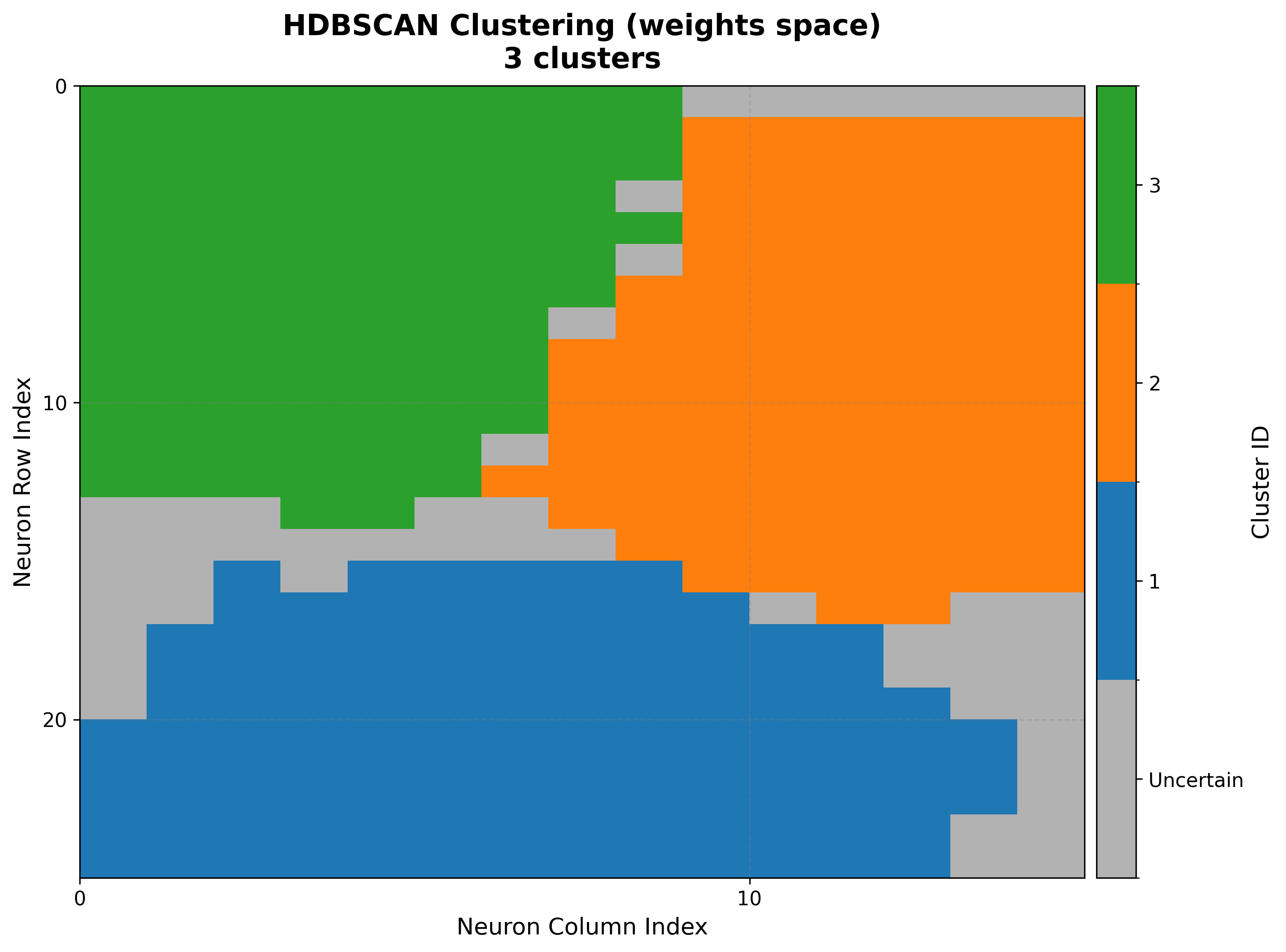
Read the cluster map together with the U-matrix: cluster boundaries should fall along the U-matrix ridges (regions of large inter-neuron distance).
End-to-end example
import torch
from sklearn.datasets import make_blobs
from sklearn.preprocessing import StandardScaler

from torchsom import SOM, SOMVisualizer

X, _ = make_blobs(n_samples=1000, centers=4, n_features=5, random_state=42)
data = torch.tensor(StandardScaler().fit_transform(X), dtype=torch.float32)

som = SOM(x=25, y=15, num_features=5, epochs=100, batch_size=16,
          topology="hexagonal", initialization_mode="pca", random_seed=42)
som.initialize_weights(data=data, mode=som.initialization_mode)
som.fit(data=data)

viz = SOMVisualizer(som=som)
viz.plot_elbow_analysis(max_k=10, feature_space="weights")     # pick k
result = som.cluster(method="kmeans", n_clusters=4, feature_space="weights")
viz.plot_cluster_map(cluster_result=result)
Next steps
Clustering — Synthetic Blobs — A full clustering tutorial on synthetic blobs
Visualization Gallery — All clustering diagnostics with example figures
Utilities API — Clustering and metric utilities