Boston Housing — Regression

The Boston Housing dataset (506 samples, 13 numeric features, one continuous target) is a standard regression benchmark. The target MEDV is the median home value. This tutorial trains a map, checks convergence, and reads the structure through the U-matrix and hit map, then turns to the regression-specific views: the mean and std target maps, the score map, and the rank map.

Note

Full runnable notebook: notebooks/boston_housing.ipynb. The figures below are its outputs.

1. Load and standardize the data

The dataset ships in the repo as a CSV. The features are every column except the last; MEDV is the continuous target. The BMU search compares raw feature distances, so standardizing the features is essential.

import torch
import pandas as pd
from sklearn.preprocessing import StandardScaler

# boston_housing.csv ships in the repo under data/notebooks/
df = pd.read_csv("data/notebooks/boston_housing.csv")

feature_df = df.iloc[:, :-1]          # all columns except the last
target_series = df.iloc[:, -1]        # last column: MEDV

features = torch.tensor(
    StandardScaler().fit_transform(feature_df), dtype=torch.float32
)
targets = torch.tensor(target_series.values, dtype=torch.float32)   # continuous
feature_names = list(feature_df.columns)

2. Train the SOM

from torchsom import SOM

som = SOM(
    x=25,
    y=15,
    num_features=features.shape[1],
    epochs=100,
    batch_size=16,
    sigma=1.45,
    learning_rate=0.95,
    neighborhood_order=3,
    topology="rectangular",
    initialization_mode="pca",
    random_seed=42,
)
som.initialize_weights(data=features, mode=som.initialization_mode)
q_errors, t_errors = som.fit(data=features)

3. Check convergence

from torchsom import SOMVisualizer

viz = SOMVisualizer(som=som)
viz.plot_training_errors(
    quantization_errors=q_errors, topographic_errors=t_errors
)

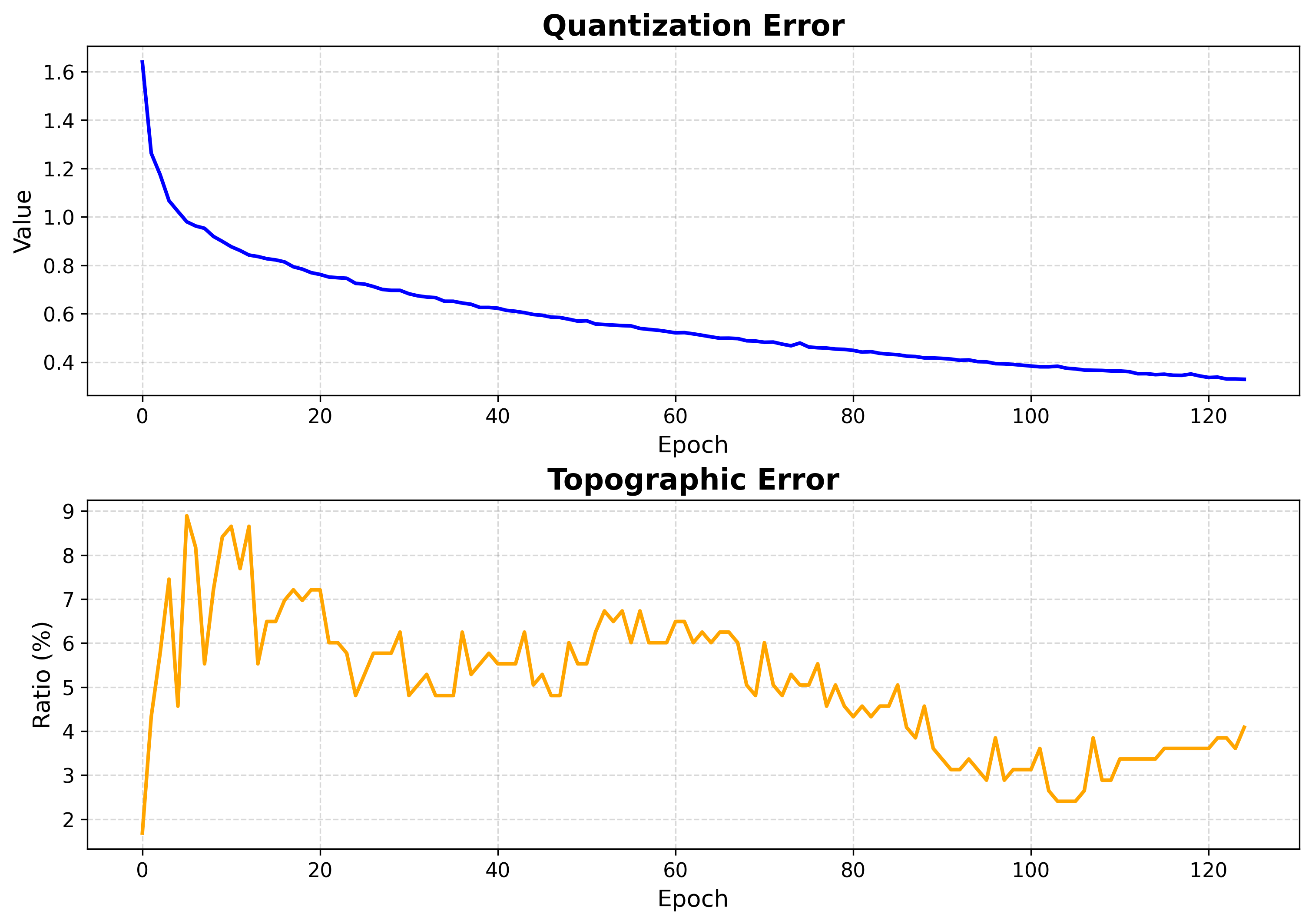
Both errors fall and flatten — training is long enough.

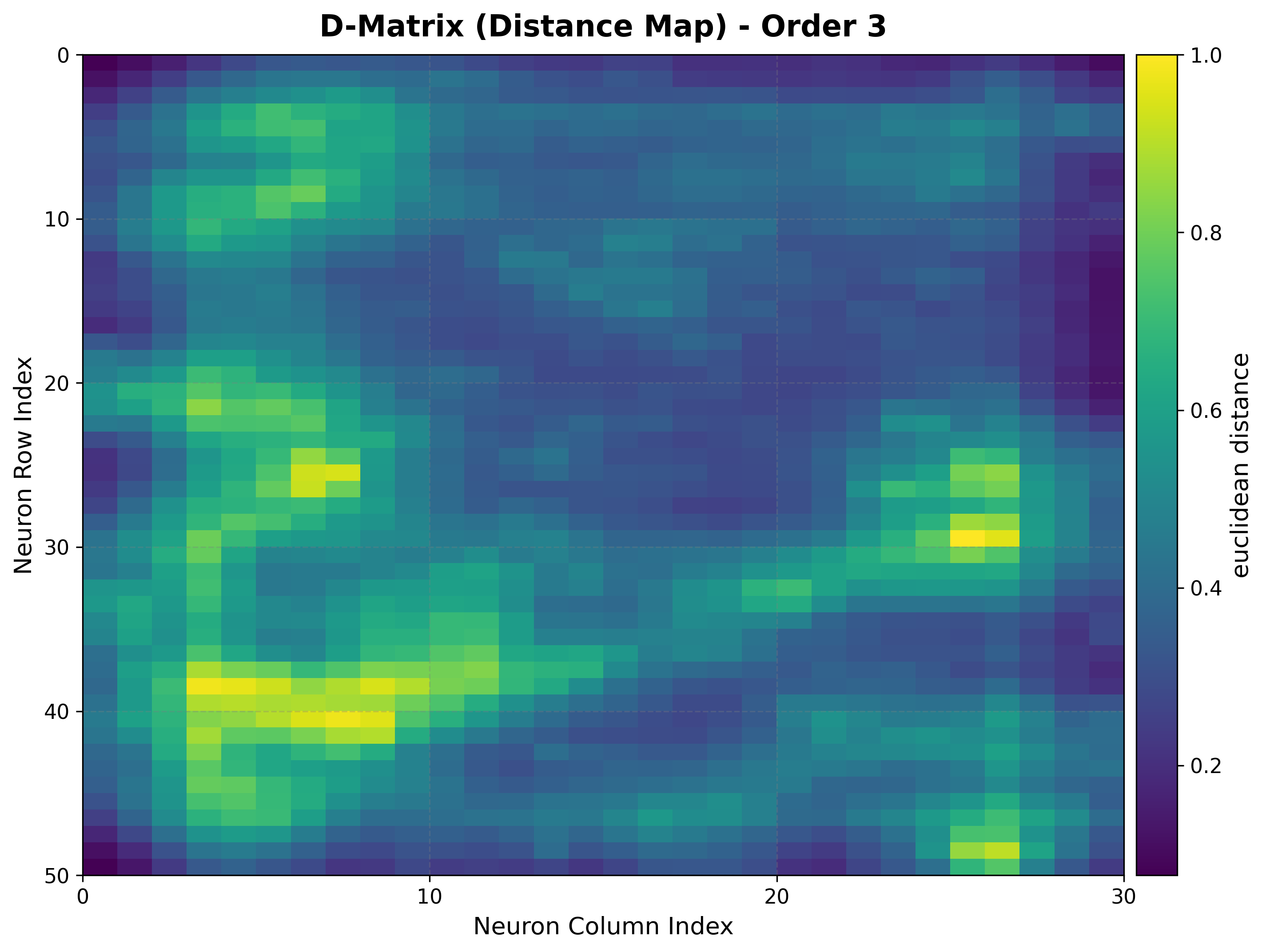
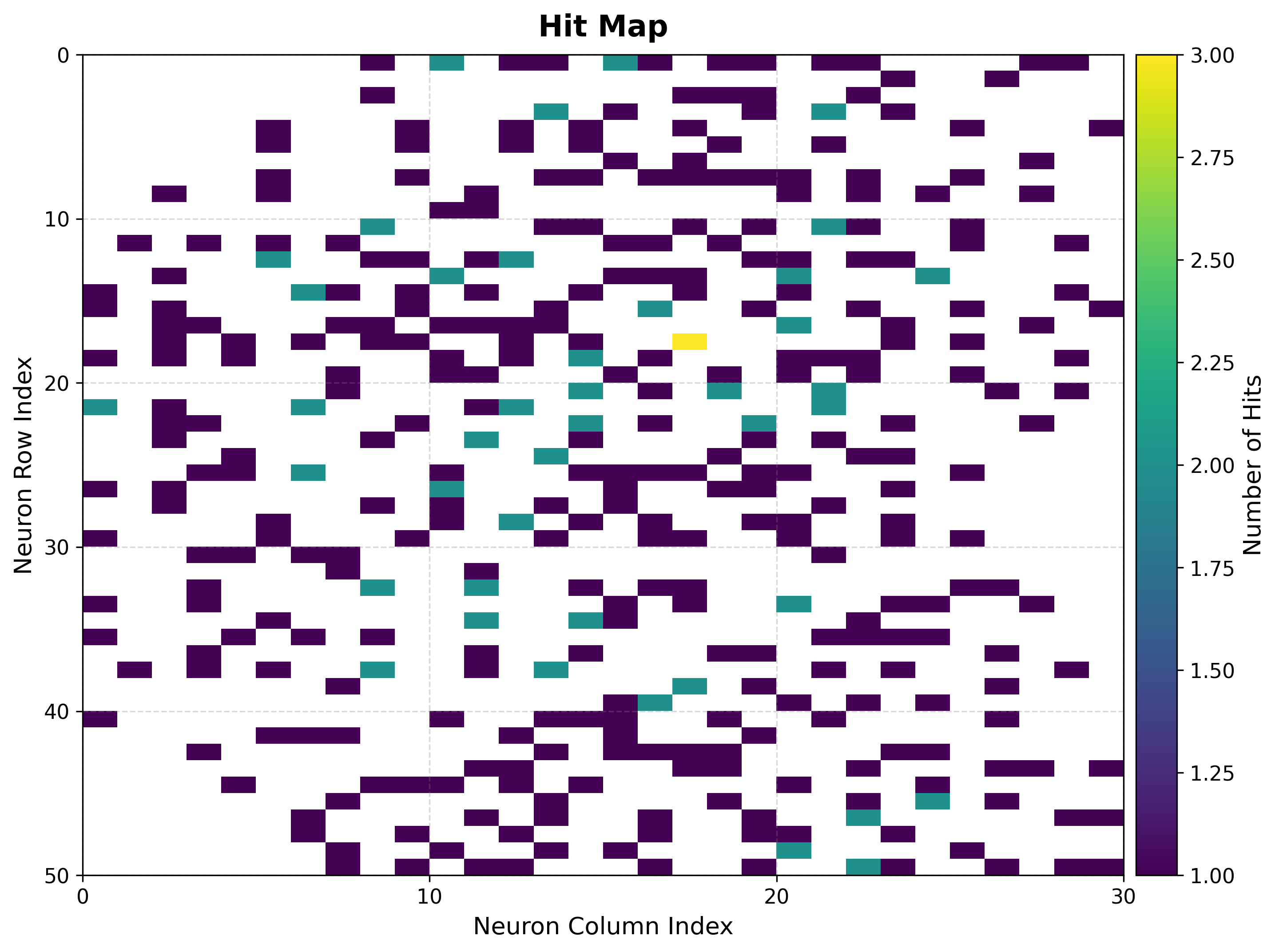
4. Map structure

The U-matrix exposes cluster boundaries; the hit map shows where the data lands.

viz.plot_distance_map(
    distance_metric=som.distance_fn_name,
    neighborhood_order=som.neighborhood_order,
)
viz.plot_hit_map(data=features)

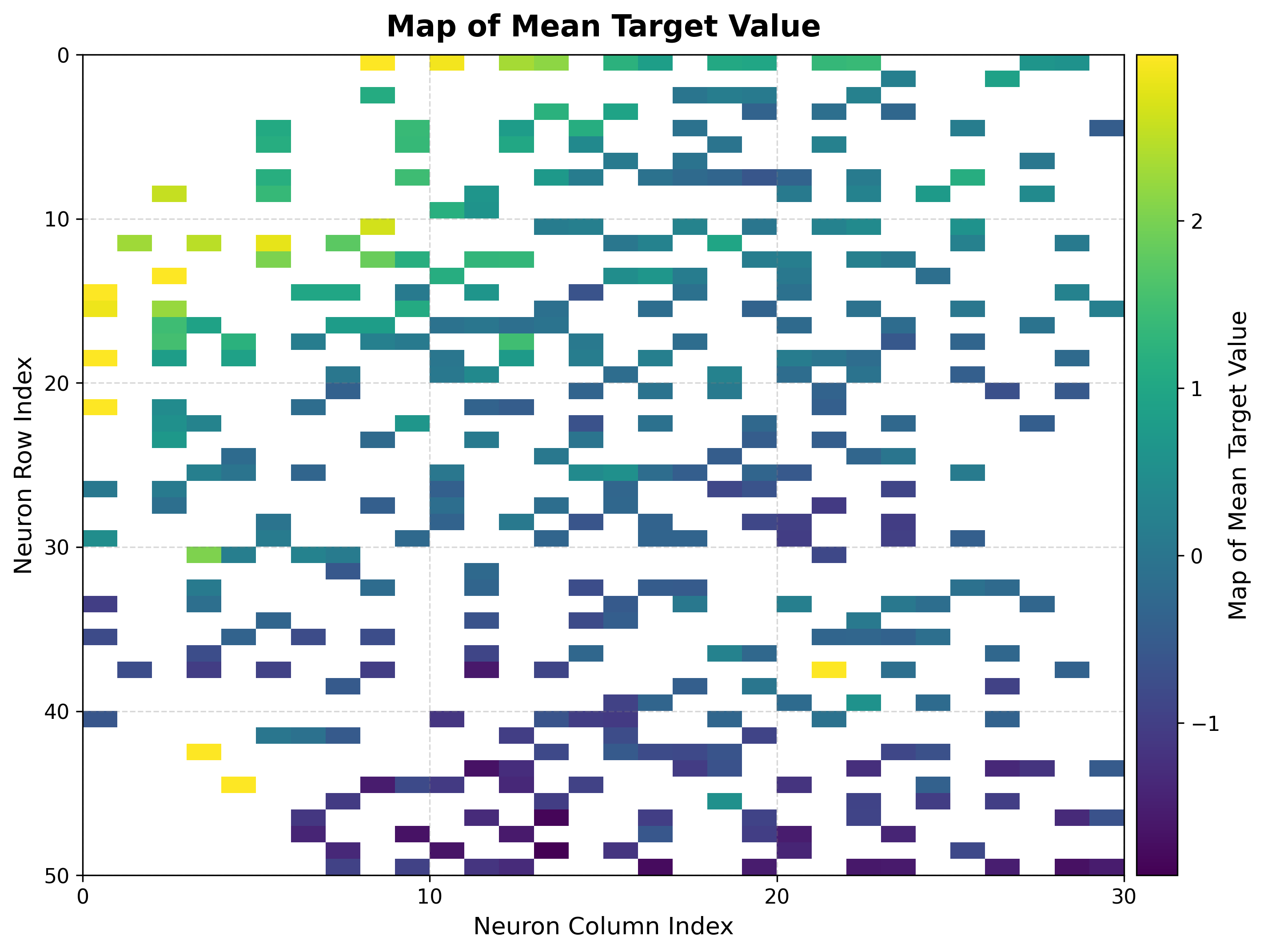
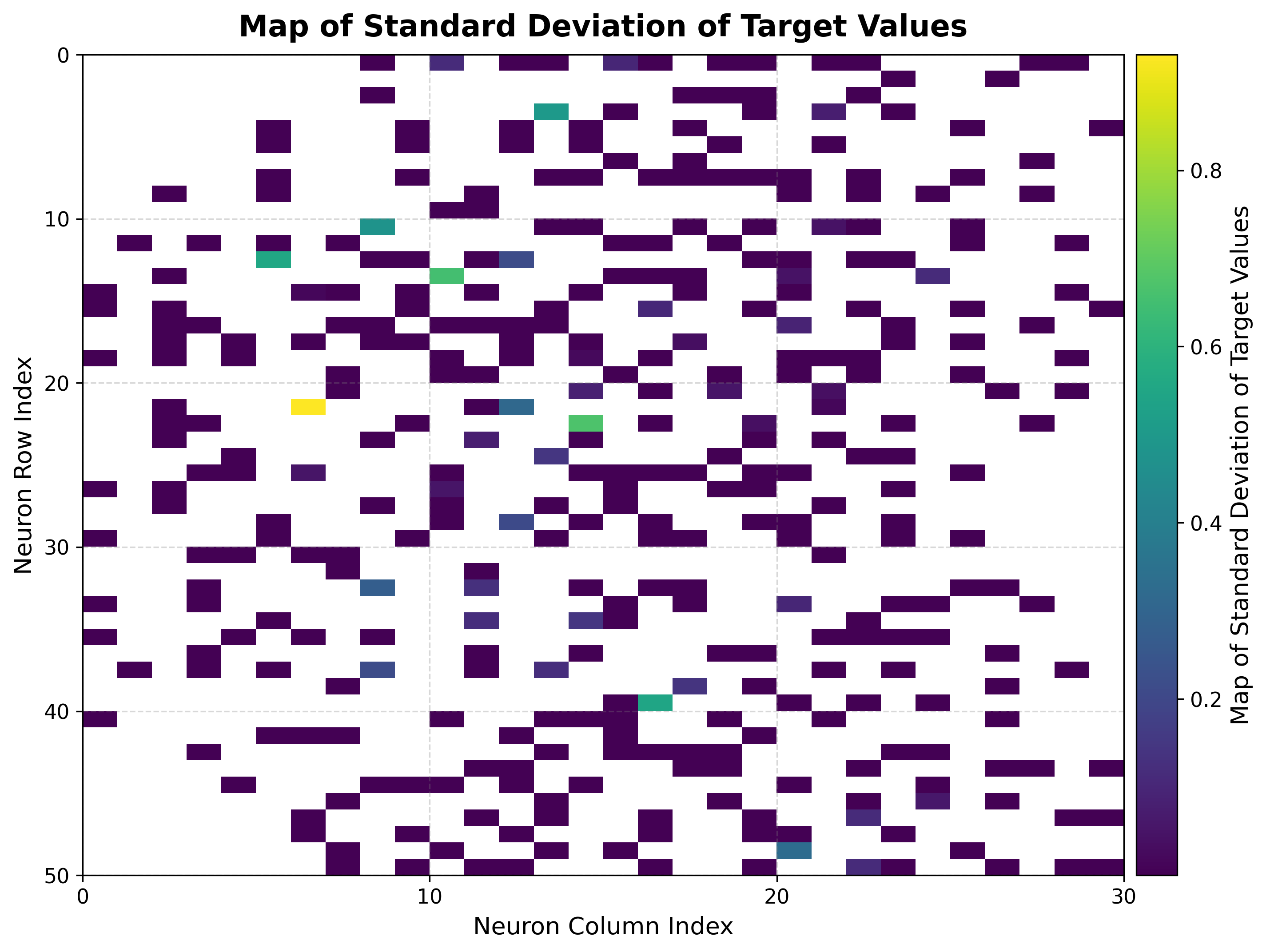
5. Target landscape

Build the BMU→sample map once, then summarize the target over each neuron. The mean map is a smooth regression surface over the topology: neighboring neurons hold similar predicted values. The std map flags neurons whose mapped samples disagree on the target, marking regions where a single prediction is less trustworthy.

bmus_map = som.build_map("bmus_data", data=features)
viz.plot_metric_map(
    bmus_data_map=bmus_map,
    data=features,
    target=targets,
    reduction_parameter="mean",
)
viz.plot_metric_map(
    bmus_data_map=bmus_map,
    data=features,
    target=targets,
    reduction_parameter="std",
)

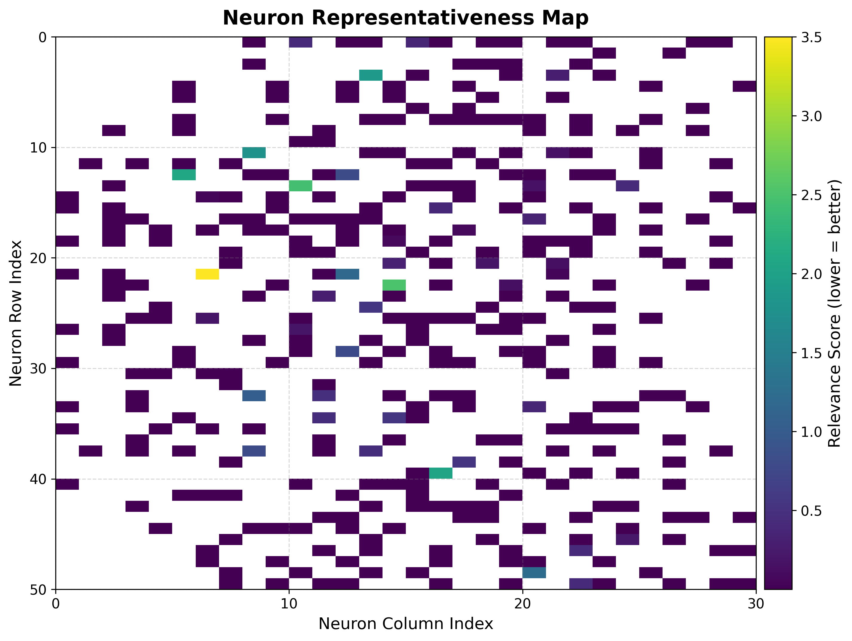
6. Per-neuron reliability

The score map combines target variance, sample count, and statistical significance into a single value where lower is better. The rank map orders neurons by std, so rank 1 is the lowest-std, most reliable neuron. Together they pinpoint which neurons give trustworthy regression estimates.

viz.plot_score_map(
    bmus_data_map=bmus_map,
    target=targets,
    total_samples=features.shape[0],
)
viz.plot_rank_map(bmus_data_map=bmus_map, target=targets)

Next steps

• Energy Efficiency — Multi-target Regression — Another regression example

• Visualization Gallery — Every plot explained

• Clustering — Group neurons into clusters