Clustering — Synthetic Blobs
Synthetic blobs (300 samples, 4 features, 3 well-separated Gaussian clusters) make the full clustering workflow easy to follow. This tutorial trains a map, picks the number of clusters with the elbow and silhouette diagnostics, clusters the neurons, draws the cluster map, and compares the three algorithms objectively. The integer blob ids serve as a known ground-truth class for the classification map.
Note
Full runnable notebook: notebooks/clustering.ipynb. The figures below are its outputs.
1. Generate and standardize the data
The BMU search compares raw feature distances, so standardizing is essential.
import torch
from sklearn.datasets import make_blobs
from sklearn.preprocessing import StandardScaler

X, y = make_blobs(n_samples=300, centers=3, n_features=4, random_state=42)
features = torch.tensor(
    StandardScaler().fit_transform(X), dtype=torch.float32
)
targets = torch.tensor(y, dtype=torch.long)   # 0, 1, 2
2. Train the SOM
from torchsom import SOM

som = SOM(
    x=25,
    y=15,
    num_features=features.shape[1],
    epochs=100,
    batch_size=16,
    sigma=1.45,
    learning_rate=0.95,
    neighborhood_order=3,
    topology="rectangular",
    initialization_mode="pca",
    random_seed=42,
)
som.initialize_weights(data=features, mode=som.initialization_mode)
q_errors, t_errors = som.fit(data=features)
3. Check convergence
from torchsom import SOMVisualizer

viz = SOMVisualizer(som=som)
viz.plot_training_errors(
    quantization_errors=q_errors, topographic_errors=t_errors
)
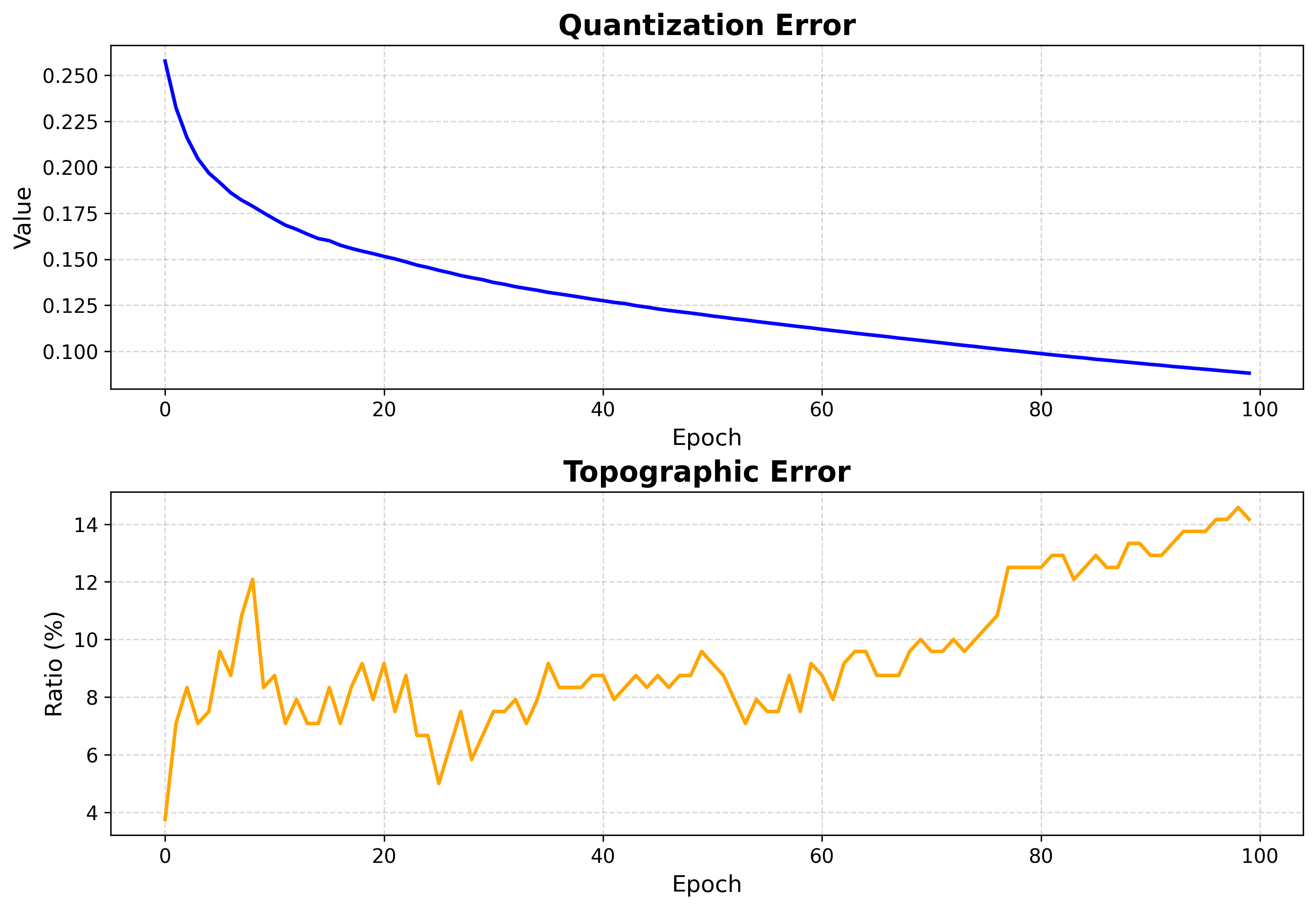
Both errors fall and flatten — training is long enough.
4. Map structure
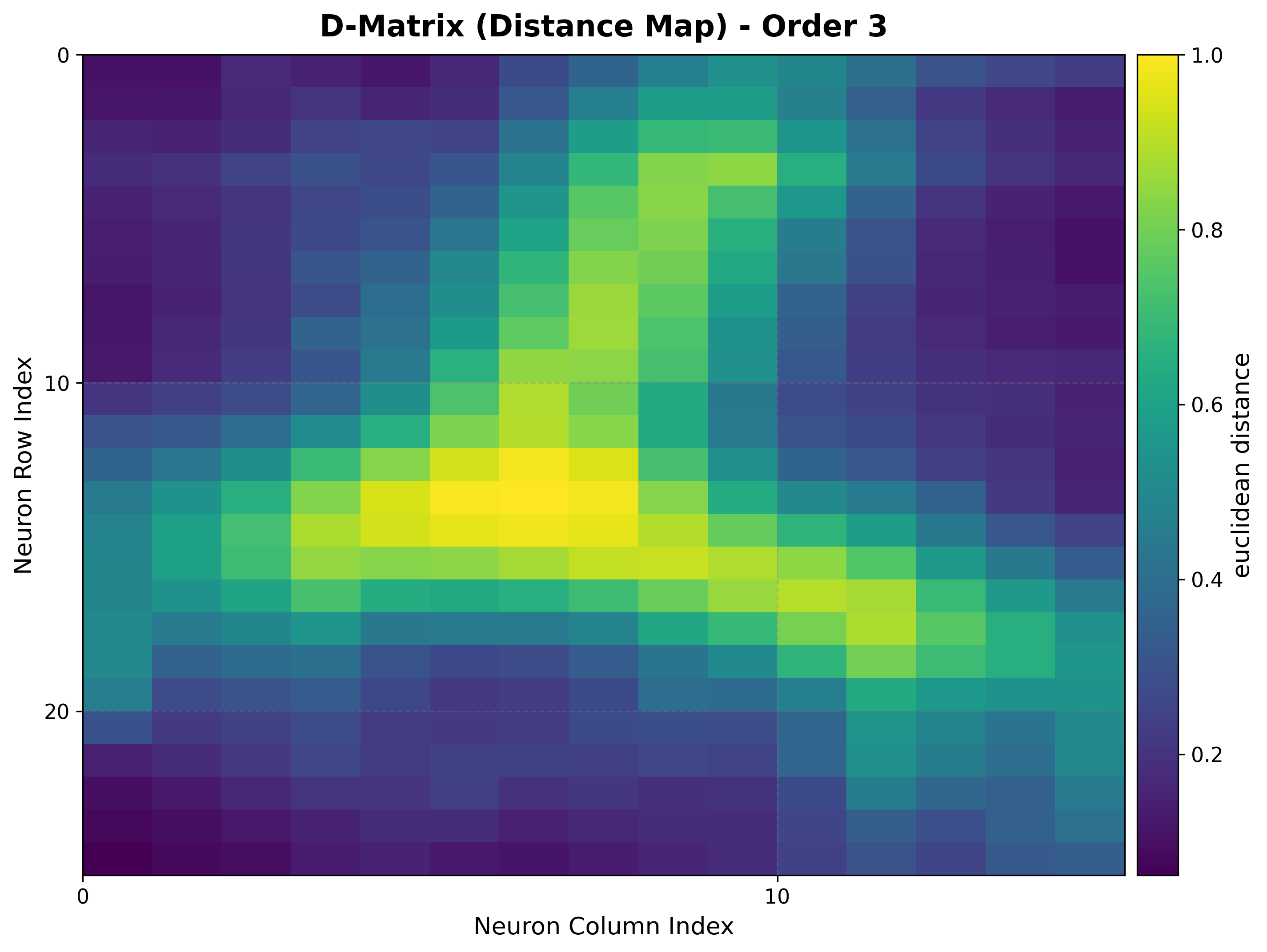
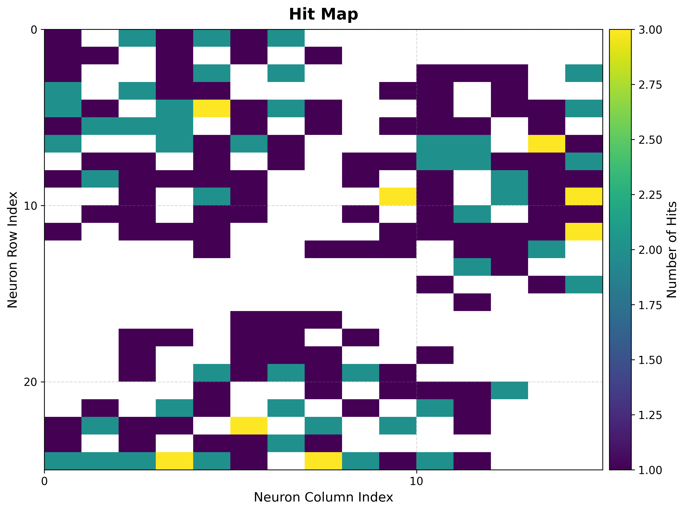
The U-matrix exposes cluster boundaries; the hit map shows where the data lands.
viz.plot_distance_map(
    distance_metric=som.distance_fn_name,
    neighborhood_order=som.neighborhood_order,
)
viz.plot_hit_map(data=features)
|
|
The U-matrix shows three basins of low inter-neuron distance separated by clear ridges, matching the three Gaussian clusters in the data.
5. Ground-truth classes
Build the BMU→sample map once, then color each neuron by its dominant blob id.
bmus_map = som.build_map("bmus_data", data=features)
viz.plot_classification_map(
    bmus_data_map=bmus_map,
    data=features,
    target=targets,
    neighborhood_order=som.neighborhood_order,
)
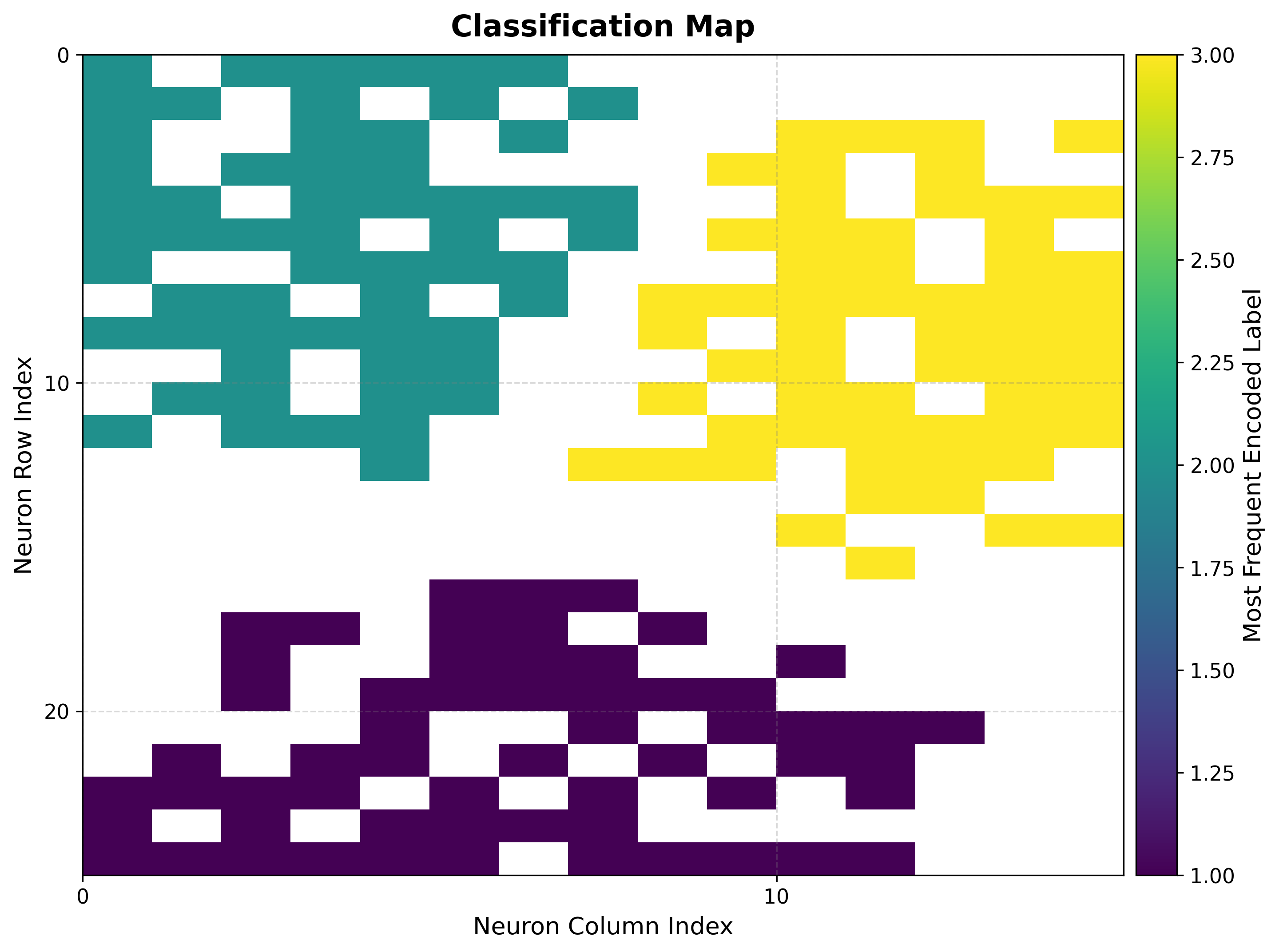
The three blobs occupy distinct, contiguous regions of the grid, confirming the map has preserved the cluster structure.
6. Choose the number of clusters
The elbow plot tracks within-cluster dispersion against k; the bend marks a good
choice.
viz.plot_elbow_analysis(max_k=10, feature_space="weights")
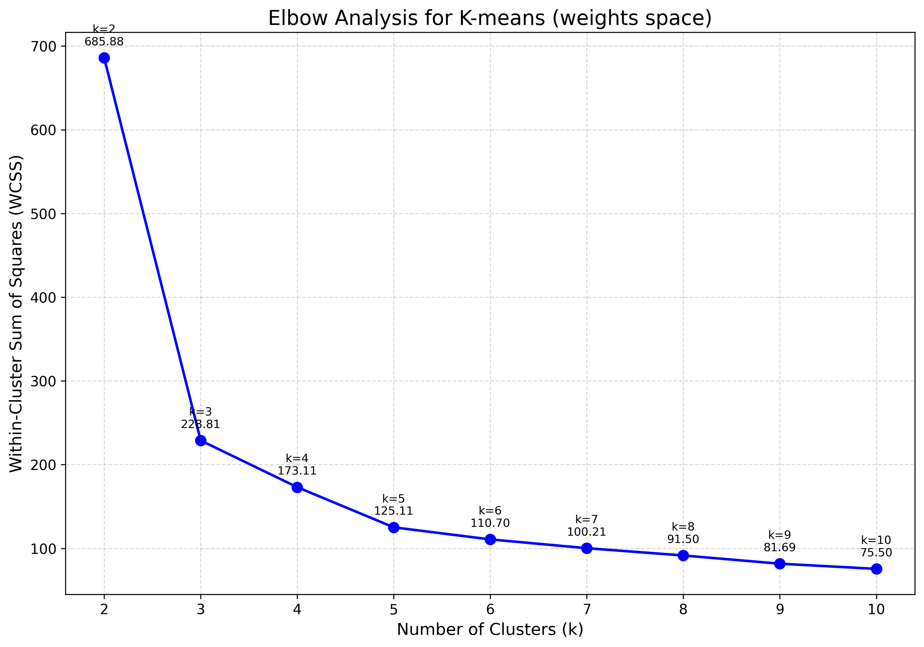
The curve bends sharply at k=3, agreeing with the three basins seen in the U-matrix.
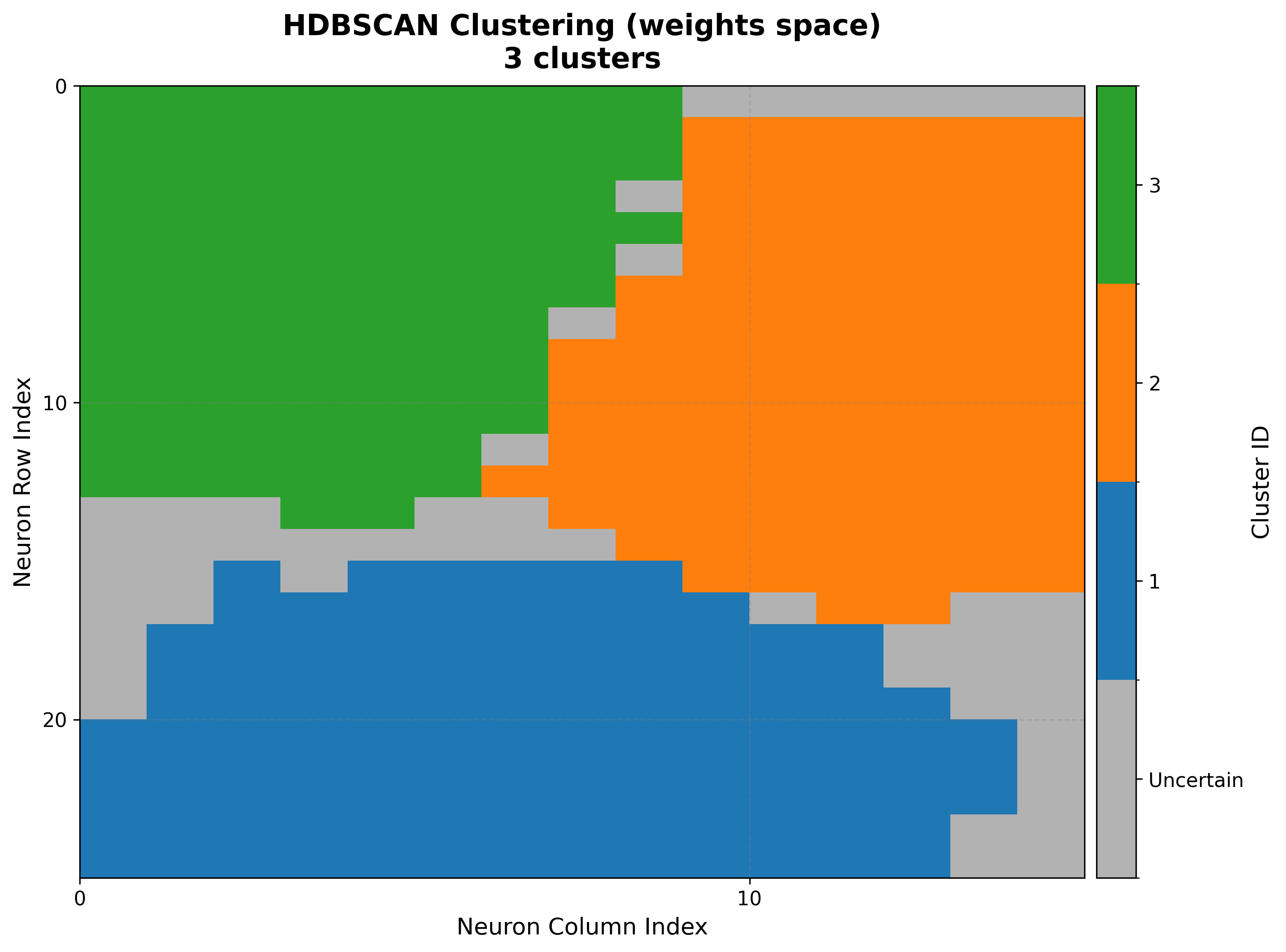
7. Cluster the neurons
With k=3 chosen, cluster the codebook vectors and draw the result.
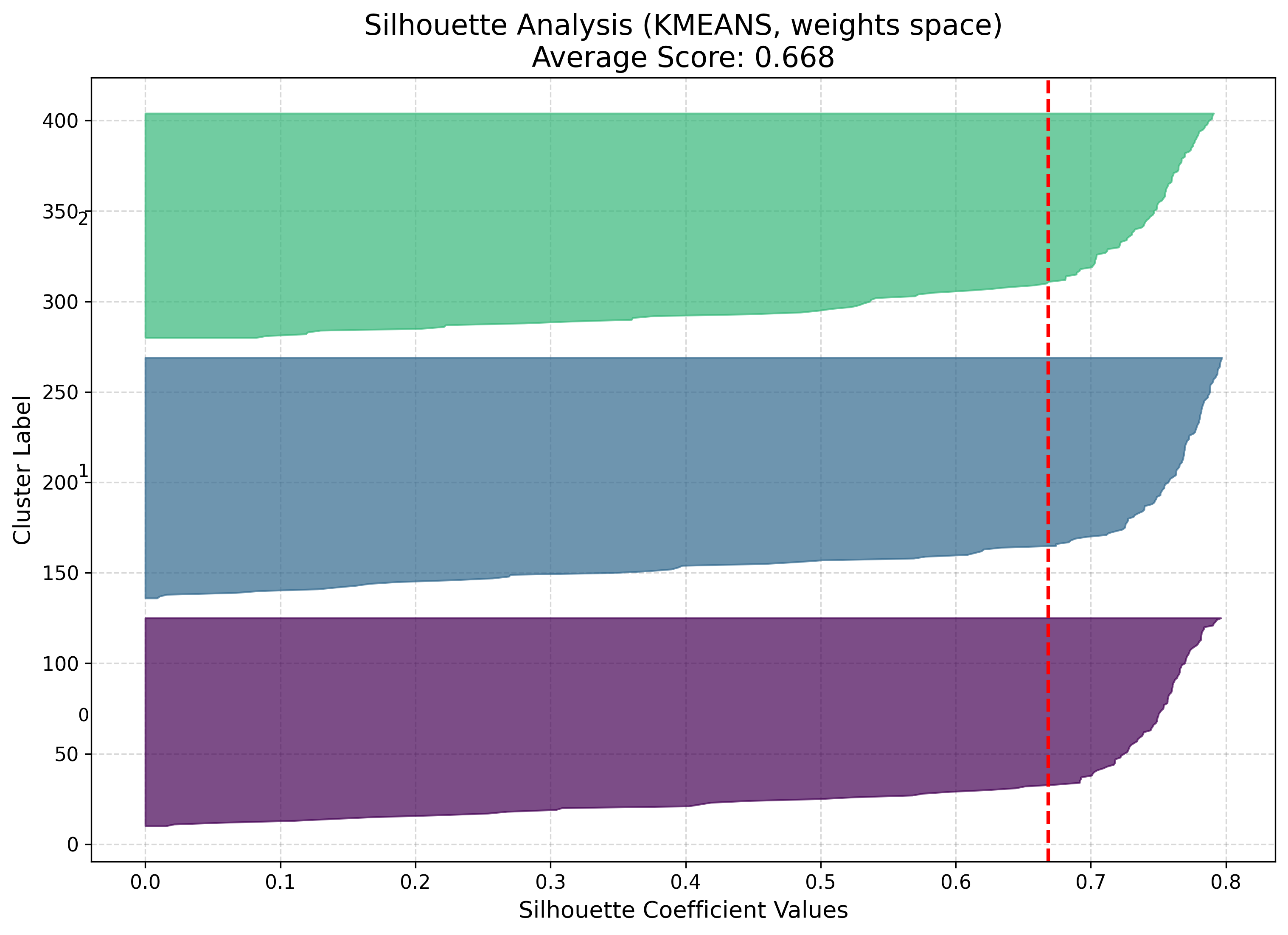
cluster() returns a dictionary; pass it straight to the
visualizer. The silhouette plot reports how cleanly each neuron sits in its cluster.
result = som.cluster(method="kmeans", n_clusters=3, feature_space="weights")
viz.plot_cluster_map(cluster_result=result)
viz.plot_silhouette_analysis(cluster_result=result)
|
|
The cluster map’s boundaries follow the U-matrix ridges, so the three neuron groups
line up with the data’s natural separation. feature_space can be "weights",
"positions", or "combined" — see Clustering for the
trade-offs.
8. Compare algorithms
Rather than picking by eye, score K-Means, GMM, and HDBSCAN side by side. n_clusters
is ignored by HDBSCAN, which finds k itself.
results = [
    som.cluster(method=m, feature_space="weights")
    for m in ("kmeans", "gmm", "hdbscan")
]
viz.plot_cluster_quality_comparison(results_list=results)
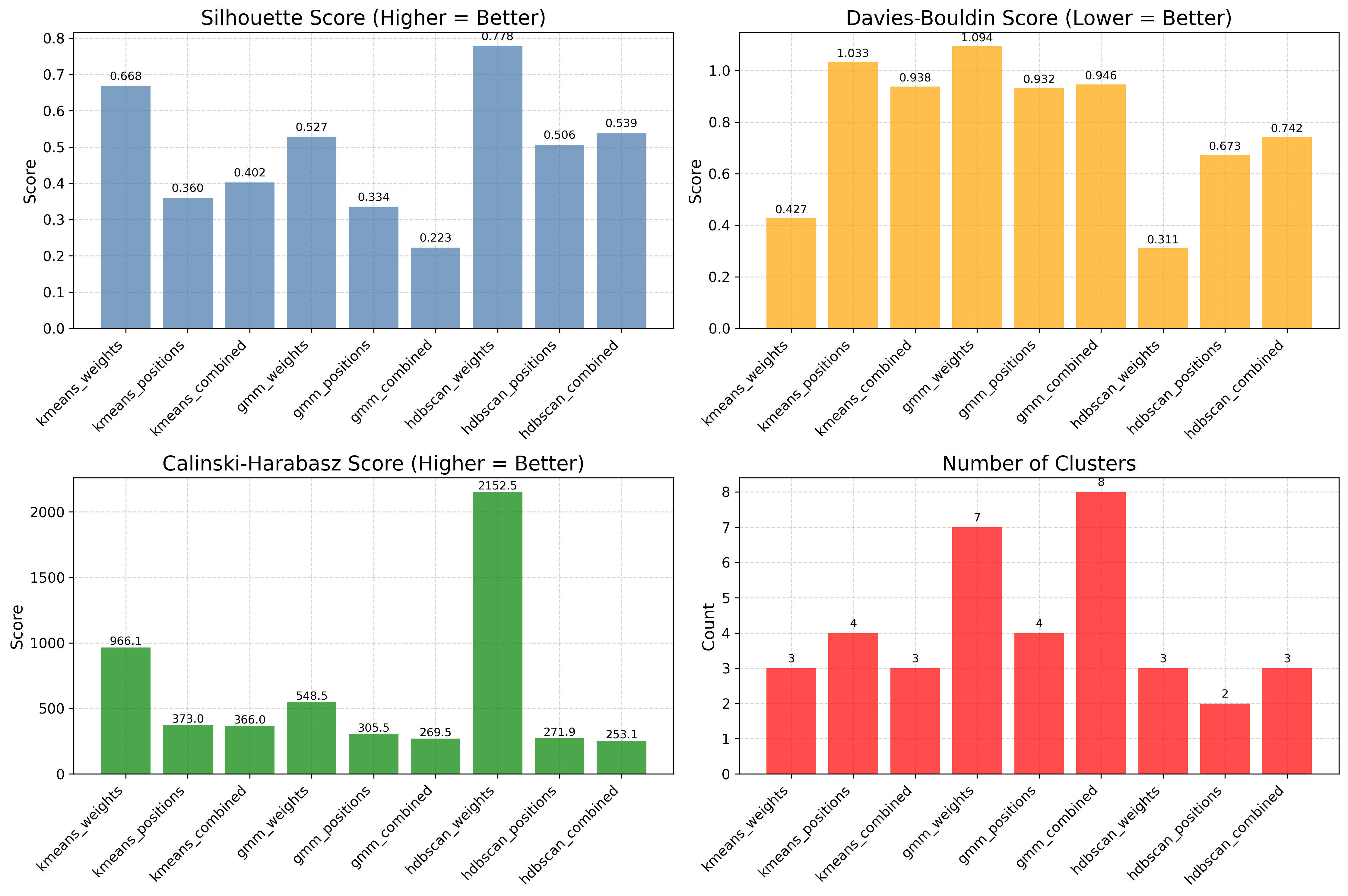
The panel scores each method with silhouette, Davies–Bouldin, and Calinski–Harabasz, so the final choice is driven by metrics rather than appearance.
Next steps
Clustering — The clustering API and feature spaces in full
Visualization Gallery — Every plot explained
Iris — Classification — A classification tutorial on the Iris dataset