Wine — Classification¶

The Wine dataset (178 samples, 13 chemical features, 3 cultivars) is a higher-dimensional classification example than iris. This tutorial trains a map, checks convergence, and reads the structure through the U-matrix, hit map, classification map, and component planes.

Note

Full runnable notebook: notebooks/wine.ipynb. The figures below are its outputs.

1. Load and standardize the data¶

The 13 chemical features span very different scales, so standardizing is essential before the BMU search compares raw feature distances.

import torch
from sklearn.datasets import load_wine
from sklearn.preprocessing import StandardScaler

bunch = load_wine()
features = torch.tensor(
    StandardScaler().fit_transform(bunch.data), dtype=torch.float32
)
targets = torch.tensor(bunch.target, dtype=torch.long)   # 0, 1, 2
feature_names = list(bunch.feature_names)

2. Train the SOM¶

from torchsom import SOM

som = SOM(
    x=25,
    y=15,
    num_features=features.shape[1],
    epochs=100,
    batch_size=16,
    sigma=1.45,
    learning_rate=0.95,
    neighborhood_order=3,
    topology="rectangular",
    initialization_mode="pca",
    random_seed=42,
)
som.initialize_weights(data=features, mode=som.initialization_mode)
q_errors, t_errors = som.fit(data=features)

3. Check convergence¶

from torchsom import SOMVisualizer

viz = SOMVisualizer(som=som)
viz.plot_training_errors(
    quantization_errors=q_errors, topographic_errors=t_errors
)

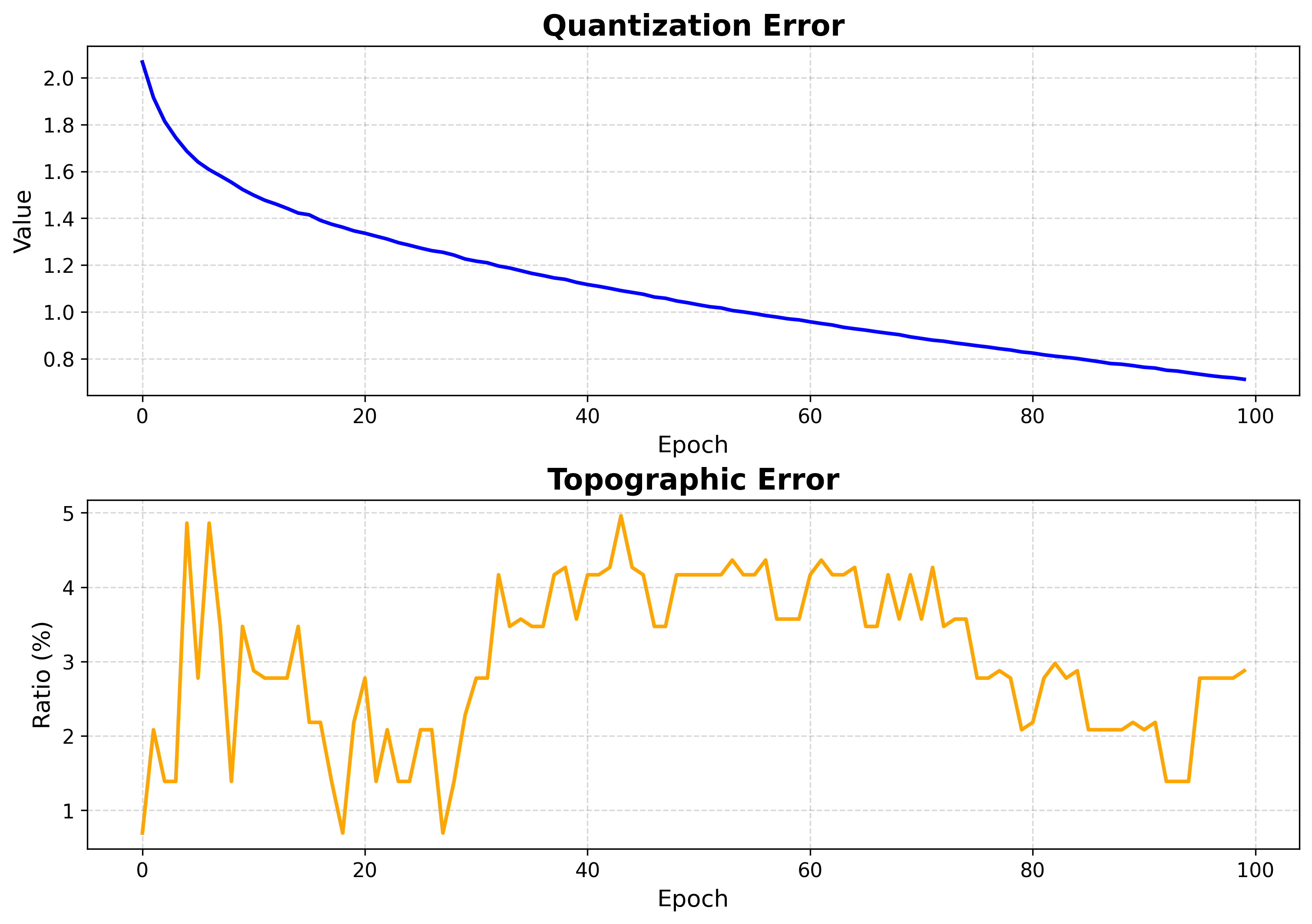
Both errors fall and flatten — training is long enough.

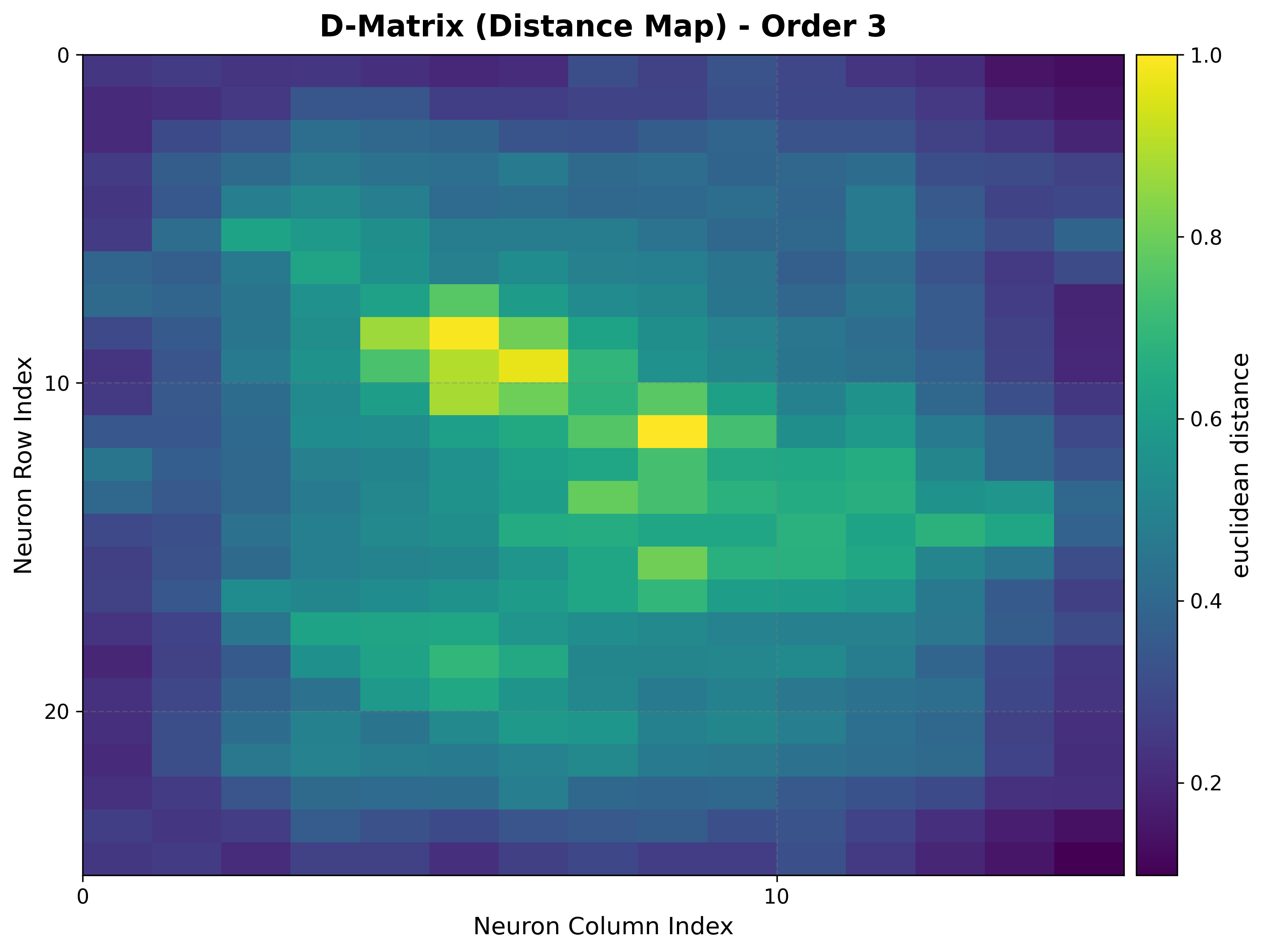
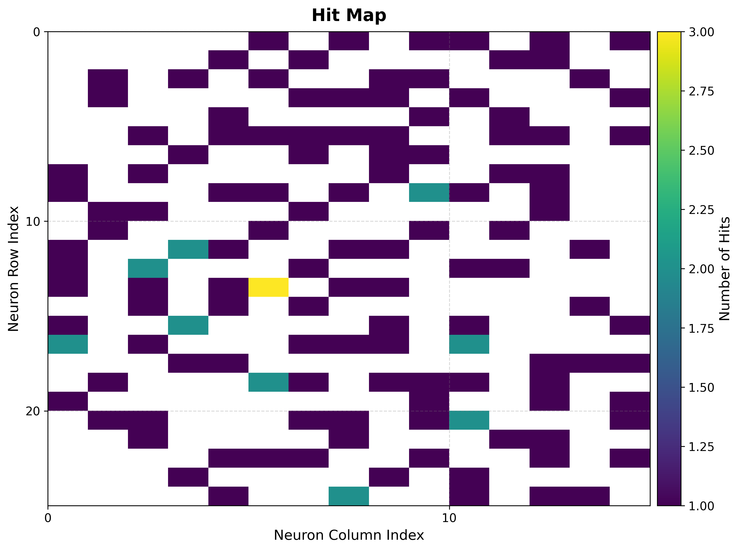
4. Inspect the map structure¶

The U-matrix exposes cluster boundaries; the hit map shows where the data lands.

viz.plot_distance_map(
    distance_metric=som.distance_fn_name,
    neighborhood_order=som.neighborhood_order,
)
viz.plot_hit_map(data=features)

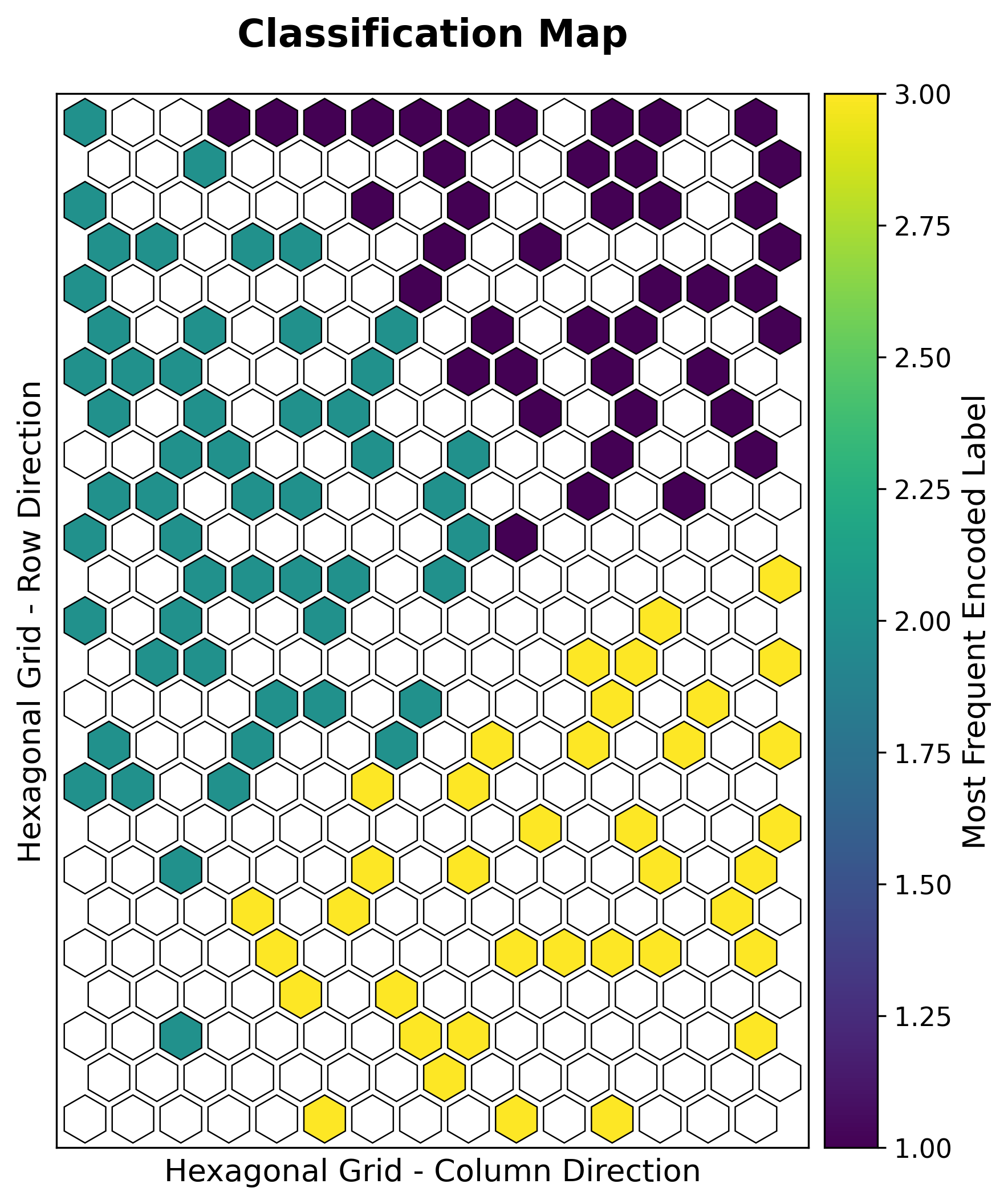
5. Classification map¶

Build the BMU→sample map once, then color each neuron by its dominant class.

bmus_map = som.build_map("bmus_data", data=features)
viz.plot_classification_map(
    bmus_data_map=bmus_map,
    data=features,
    target=targets,
    neighborhood_order=som.neighborhood_order,
)

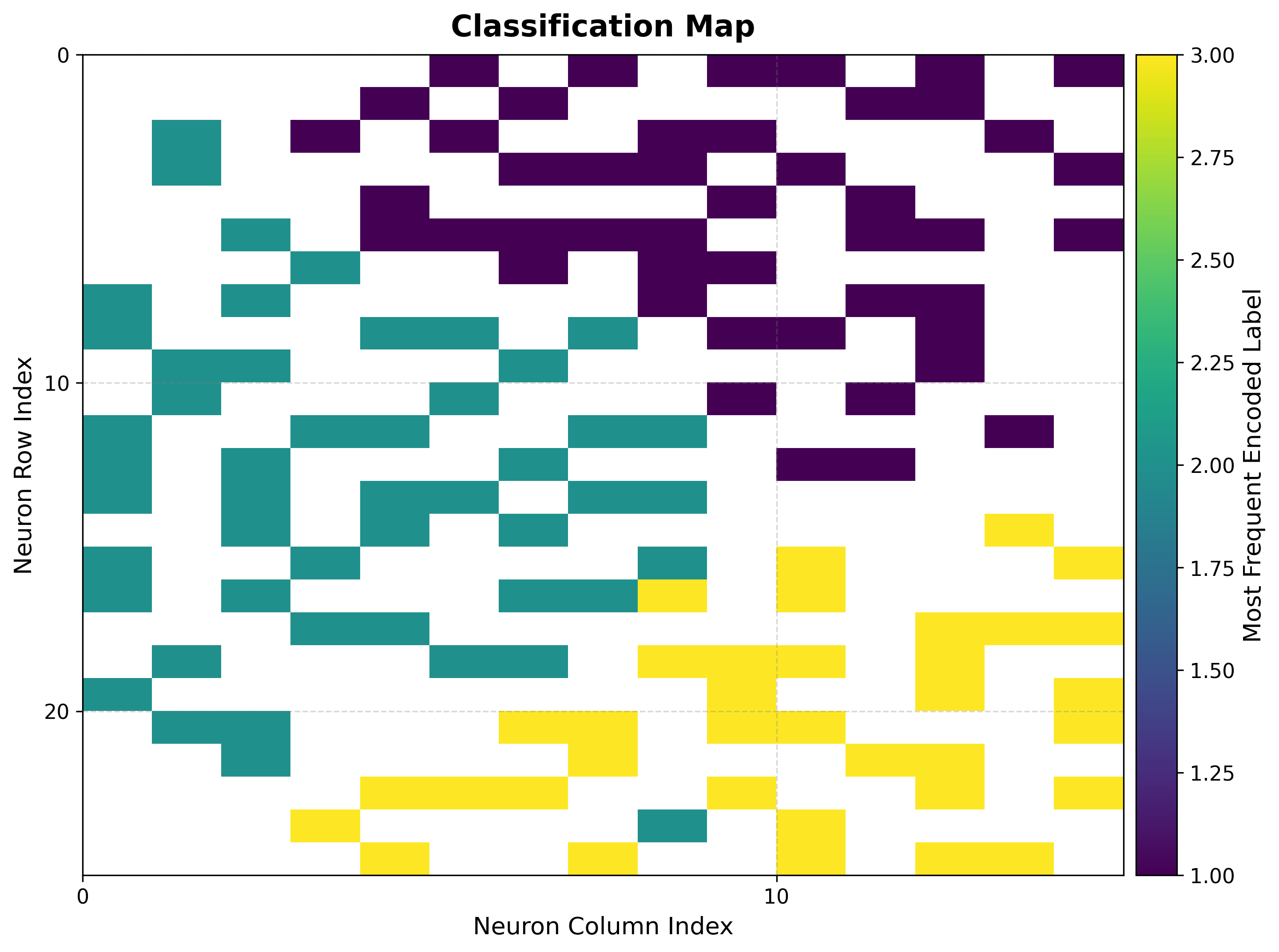
The three cultivars occupy distinct regions of the grid. The 13 features give a clearer 3-class separation than iris, with little overlap between the classes.

6. Component planes¶

One heat map per feature reveals which features drive the separation. With 13 features there is one plane per feature; see the notebook for the full set.

viz.plot_component_planes(component_names=feature_names)

The planes that vary together across the grid and align with the class regions are the most discriminative chemical measurements.

Hexagonal variant¶

Set topology="hexagonal" for the same analysis on a hexagonal grid; the visualizer renders hexagon cells automatically:

Wine classification map on a hexagonal grid

Next steps¶

Iris — Classification — The classic first SOM classification example
Boston Housing — Regression — From classification to regression
Visualization Gallery — Every plot explained